Python implements ten classic sorting algorithms artipub

reference material: https://www.bilibili.com/video/BV1mp4y1D7UP
Source of dynamic diagram demonstration in this paper: https://visualgo.net/

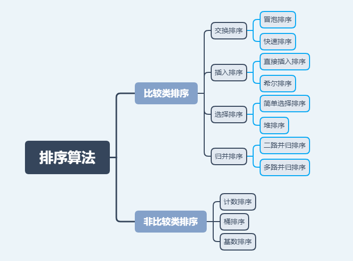
Sorting algorithm classification

Internal sort: refers to the sort in which all elements are stored in memory during sorting. Common internal sorting algorithms include bubble sort, selection sort, insertion sort, Hill sort, merge sort, quick sort, heap sort, cardinal sort, etc.
External sorting: refers to sorting in which all elements cannot be stored in memory at the same time during sorting, and must be moved between internal and external memory according to requirements during sorting;
Comparison sort: the relative order between elements is determined by comparison. Because its time complexity cannot exceed O(nlogn), it is also called nonlinear time comparison sort.
Non comparison sort: it does not determine the relative order between elements through comparison. It can break through the time lower bound based on comparison sort and run in linear time. Therefore, it is also called linear time non comparison sort. Common non comparison sorting algorithms include cardinality sorting, counting sorting, bucket sorting, etc

Generally, there are two operations in the execution of internal sorting algorithm: comparison and movement. By comparing the size of the two keywords, the relationship between the corresponding elements is determined, and then the elements are moved to achieve order. However, not all internal sorting algorithms are based on comparison operations.

Each sorting algorithm has its own advantages and disadvantages, and is suitable for use in different environments. In terms of its overall performance, it is difficult to propose the best algorithm. Generally, sorting algorithms can be divided into five categories: insertion sorting, exchange sorting, selection sorting, merge sorting and cardinal sorting. The performance of internal sorting algorithms depends on the time complexity and space complexity of the algorithm, and the time complexity is generally determined by the number of comparisons and moves.

Sorting algorithm	Time complexity (average)	Time complexity (best)	Time complexity (worst case)	Spatial complexity	stability
Bubble sorting	O ( n 2 ) O(n^2) O(n2)	O ( n ) O(n) O(n)	O ( n 2 ) O(n^2) O(n2)	O ( 1 ) O(1) O(1)	stable
Select sort	O ( n 2 ) O(n^2) O(n2)	O ( n 2 ) O(n^2) O(n2)	O ( n 2 ) O(n^2) O(n2)	O ( 1 ) O(1) O(1)	instable
Insert sort	O ( n 2 ) O(n^2) O(n2)	O ( n ) O(n) O(n)	O ( n 2 ) O(n^2) O(n2)	O ( 1 ) O(1) O(1)	stable
Shell Sort	O ( n l o g n ) O(nlogn) O(nlogn)	O ( n l o g 2 n ) O(nlog^2n) O(nlog2n)	O ( n l o g 2 n ) O(nlog^2n) O(nlog2n)	O ( 1 ) O(1) O(1)	instable
Merge sort	O ( n l o g n ) O(nlogn) O(nlogn)	O ( n l o g n ) O(nlogn) O(nlogn)	O ( n l o g n ) O(nlogn) O(nlogn)	O ( n ) O(n) O(n)	stable
Quick sort	O ( n l o g n ) O(nlogn) O(nlogn)	O ( n l o g n ) O(nlogn) O(nlogn)	O ( n 2 ) O(n^2) O(n2)	O ( l o g n ) O(logn) O(logn)	instable
Heap sort	O ( n l o g n ) O(nlogn) O(nlogn)	O ( n l o g n ) O(nlogn) O(nlogn)	O ( n l o g n ) O(nlogn) O(nlogn)	O ( 1 ) O(1) O(1)	instable
Count sort	O ( n + k ) O(n+k) O(n+k)	O ( n + k ) O(n+k) O(n+k)	O ( n + k ) O(n+k) O(n+k)	O ( k ) O(k) O(k)	stable
Bucket sorting	O ( n + k ) O(n+k) O(n+k)	O ( n + k ) O(n+k) O(n+k)	O ( n 2 ) O(n^2) O(n2)	O ( n + k ) O(n+k) O(n+k)	stable
Cardinality sort	O ( n ∗ k ) O(n*k) O(n∗k)	O ( n ∗ k ) O(n*k) O(n∗k)	O ( n ∗ k ) O(n*k) O(n∗k)	O ( n + k ) O(n+k) O(n+k)	stable

Stability: whether the order of the two equal key values after sorting is the same as that before sorting. For example, if a was originally in front of b, and a=b, and a is still in front of b after sorting, it indicates stability.

Comparison of common time complexity:

O ( 1 ) < O ( l o g n ) < O ( n ) < O ( n l o g n ) < O ( n 2 ) < . . . < O ( 2 n ) < O ( n ! ) O(1) < O(logn) < O(n) < O(nlogn) < O(n^2) <...< O(2^n)<O (n!) O(1)<O(logn)<O(n)<O(nlogn)<O(n2)<...<O(2n)<O(n!)

1, Bubble Sort

1. Principle

Repeatedly visit the elements to be sorted, compare two adjacent elements in turn, and exchange them if the order (e.g. from large to small) is wrong. The work of visiting elements is repeated until no adjacent elements need to be exchanged, that is, the element column has been sorted. Bubbling actually means that each round of bubbling, the largest element will move to the far right by constantly comparing and exchanging adjacent elements.

If there are 10 small basin friends standing in a row from left to right, their sizes vary. The teacher wanted them to stand from low to high, so he began to shout slogans. Each time, starting from the first child, the neighboring children will exchange in pairs if their height is not in positive order. In this way, the highest child in the first round will be ranked to the right (bubbling to the right). In the second round, they will exchange in pairs from the first child, so that the second highest child will be ranked to the penultimate position. And so on.

2. Steps

① Compare adjacent elements. If the first is bigger than the second, exchange them two;
② Do the same for each pair of adjacent elements, from the first pair at the beginning to the last pair at the end, so that the last element should be the largest number;
③ Repeat steps ① ~ ② for all elements except the last element until the sorting is completed.

3. Animation demonstration

4. Code implementation

def bubbleSort(arr):
    for i in range(len(arr)-1):         # Cycle i
        for j in range(len(arr)-i-1):   # j is the subscript
            if arr[j] > arr[j+1]:       # If this number is greater than the following number, swap the positions of the two
                arr[j], arr[j+1] = arr[j+1], arr[j]
    return arr

Another optimization algorithm for bubble sorting is to set up a flag. When there is no exchange of elements in a sequence traversal, it is proved that the sequence has been ordered and no subsequent sorting will be carried out. The improved algorithm is shown in the animation demonstration. The improved code is as follows:

def bubbleSort(arr):
    for i in range(len(arr)-1):         # Cycle i
    flag = False
        for j in range(len(arr)-i-1):   # j is the subscript
            if arr[j] > arr[j+1]:       # If this number is greater than the following number, swap the positions of the two
                arr[j], arr[j+1] = arr[j+1], arr[j]
                flag = True
        if not flag:
            return
    return arr

Bubble sorting is the fastest: when the input data is in positive order; The slowest case: when the input data is in reverse order.

5. Specific examples

Unmodified version:

def bubble_sort(arr):
    for i in range(len(arr)-1):         # Cycle i
        for j in range(len(arr)-i-1):   # j is the subscript
            if arr[j] > arr[j+1]:       # If this number is greater than the following number, swap the positions of the two
                arr[j], arr[j+1] = arr[j+1], arr[j]
        print(arr)                      # Print once after each comparison


arr = [3, 44, 38, 5, 47, 15, 36, 26, 27, 2, 46, 4, 19, 50, 48]
bubble_sort(arr)

[3, 38, 5, 44, 15, 36, 26, 27, 2, 46, 4, 19, 47, 48, 50]
[3, 5, 38, 15, 36, 26, 27, 2, 44, 4, 19, 46, 47, 48, 50]
[3, 5, 15, 36, 26, 27, 2, 38, 4, 19, 44, 46, 47, 48, 50]
[3, 5, 15, 26, 27, 2, 36, 4, 19, 38, 44, 46, 47, 48, 50]
[3, 5, 15, 26, 2, 27, 4, 19, 36, 38, 44, 46, 47, 48, 50]
[3, 5, 15, 2, 26, 4, 19, 27, 36, 38, 44, 46, 47, 48, 50]
[3, 5, 2, 15, 4, 19, 26, 27, 36, 38, 44, 46, 47, 48, 50]
[3, 2, 5, 4, 15, 19, 26, 27, 36, 38, 44, 46, 47, 48, 50]
[2, 3, 4, 5, 15, 19, 26, 27, 36, 38, 44, 46, 47, 48, 50]
[2, 3, 4, 5, 15, 19, 26, 27, 36, 38, 44, 46, 47, 48, 50]
[2, 3, 4, 5, 15, 19, 26, 27, 36, 38, 44, 46, 47, 48, 50]
[2, 3, 4, 5, 15, 19, 26, 27, 36, 38, 44, 46, 47, 48, 50]
[2, 3, 4, 5, 15, 19, 26, 27, 36, 38, 44, 46, 47, 48, 50]
[2, 3, 4, 5, 15, 19, 26, 27, 36, 38, 44, 46, 47, 48, 50]

Improved version:

def bubble_sort(arr):
    for i in range(len(arr)-1):         # Cycle i
        flag = False
        for j in range(len(arr)-i-1):   # j is the subscript
            if arr[j] > arr[j+1]:       # If this number is greater than the following number, swap the positions of the two
                arr[j], arr[j+1] = arr[j+1], arr[j]
                flag = True
        if not flag:
            return
        print(arr)                      # Print once after each comparison


arr = [3, 44, 38, 5, 47, 15, 36, 26, 27, 2, 46, 4, 19, 50, 48]
bubble_sort(arr)

[3, 38, 5, 44, 15, 36, 26, 27, 2, 46, 4, 19, 47, 48, 50]
[3, 5, 38, 15, 36, 26, 27, 2, 44, 4, 19, 46, 47, 48, 50]
[3, 5, 15, 36, 26, 27, 2, 38, 4, 19, 44, 46, 47, 48, 50]
[3, 5, 15, 26, 27, 2, 36, 4, 19, 38, 44, 46, 47, 48, 50]
[3, 5, 15, 26, 2, 27, 4, 19, 36, 38, 44, 46, 47, 48, 50]
[3, 5, 15, 2, 26, 4, 19, 27, 36, 38, 44, 46, 47, 48, 50]
[3, 5, 2, 15, 4, 19, 26, 27, 36, 38, 44, 46, 47, 48, 50]
[3, 2, 5, 4, 15, 19, 26, 27, 36, 38, 44, 46, 47, 48, 50]
[2, 3, 4, 5, 15, 19, 26, 27, 36, 38, 44, 46, 47, 48, 50]

2, Selection Sort

1. Principle

Select the smallest (or largest) element from the data elements to be sorted for the first time, store it at the beginning of the sequence, and then find the smallest (large) element from the remaining unordered elements, and then put it at the end of the sorted sequence. And so on until the number of all data elements to be sorted is zero. It can be understood as an iteration from 0 to n-1. Each backward search selects the smallest element. Selective sorting is an unstable sorting method.

If there are 10 small basin friends standing in a row from left to right, their sizes vary. The teacher wants them to stand from low to high. We start from the first, find the smallest pot friend from beginning to end, and then exchange it with the first pot friend. Then start with the second little friend and adopt the same strategy. In this way, the little friend is orderly.

2. Steps

① First, find the smallest (large) element in the unordered sequence and store it at the beginning of the sorted sequence;
② Then continue to find the smallest (large) element from the remaining unordered elements, and then put it at the end of the sorted sequence;
③ Repeat step ② until all elements are sorted.

3. Animation demonstration

4. Code implementation

Python code:

def selection_sort(arr):
    for i in range(len(arr)-1):          # Cycle i
        min_index = i                    # Record the subscript of the lowest decimal point
        for j in range(i+1, len(arr)):   # j is the subscript
            if arr[j] < arr[min_index]:  # If this number is less than the minimum number of records, the subscript of the minimum number is updated
                min_index = j
        arr[i], arr[min_index] = arr[min_index], arr[i]  # Swap the number at i position (the number at the end of the sorted sequence) with the lowest decimal
    return arr

5. Specific examples

def selection_sort(arr):
    for i in range(len(arr)-1):          # Cycle i
        min_index = i                    # Record the subscript of the lowest decimal point
        for j in range(i+1, len(arr)):   # j is the subscript
            if arr[j] < arr[min_index]:  # If this number is less than the minimum number of records, the subscript of the minimum number is updated
                min_index = j
        arr[i], arr[min_index] = arr[min_index], arr[i]  # Swap the number at i position (the number at the end of the sorted sequence) with the lowest decimal
        print(arr)                       # Print once after each comparison


arr = [3, 44, 38, 5, 47, 15, 36, 26, 27, 2, 46, 4, 19, 50, 48]
selection_sort(arr)

[2, 44, 38, 5, 47, 15, 36, 26, 27, 3, 46, 4, 19, 50, 48]
[2, 3, 38, 5, 47, 15, 36, 26, 27, 44, 46, 4, 19, 50, 48]
[2, 3, 4, 5, 47, 15, 36, 26, 27, 44, 46, 38, 19, 50, 48]
[2, 3, 4, 5, 47, 15, 36, 26, 27, 44, 46, 38, 19, 50, 48]
[2, 3, 4, 5, 15, 47, 36, 26, 27, 44, 46, 38, 19, 50, 48]
[2, 3, 4, 5, 15, 19, 36, 26, 27, 44, 46, 38, 47, 50, 48]
[2, 3, 4, 5, 15, 19, 26, 36, 27, 44, 46, 38, 47, 50, 48]
[2, 3, 4, 5, 15, 19, 26, 27, 36, 44, 46, 38, 47, 50, 48]
[2, 3, 4, 5, 15, 19, 26, 27, 36, 44, 46, 38, 47, 50, 48]
[2, 3, 4, 5, 15, 19, 26, 27, 36, 38, 46, 44, 47, 50, 48]
[2, 3, 4, 5, 15, 19, 26, 27, 36, 38, 44, 46, 47, 50, 48]
[2, 3, 4, 5, 15, 19, 26, 27, 36, 38, 44, 46, 47, 50, 48]
[2, 3, 4, 5, 15, 19, 26, 27, 36, 38, 44, 46, 47, 50, 48]
[2, 3, 4, 5, 15, 19, 26, 27, 36, 38, 44, 46, 47, 48, 50]

3, Insertion Sort

1. Principle

Insert sort is also commonly referred to as direct insert sort. It is an effective algorithm for sorting a small number of elements. Its basic idea is to insert a record into the ordered table, so as to form a new ordered table. In its implementation process, a double-layer loop is used. The outer loop traverses all elements except the first element, and the inner loop looks up the position to be inserted in the ordered table in front of the current element and moves it.

Insert sort works like many people sort a hand of playing cards. At first, our left hand is empty and the cards on the table face down. Then, we take a card from the table one at a time and insert it in the correct position in our left hand. In order to find the correct position of a card, we compare it from right to left with each card already in hand. The cards on the left hand are always sorted. It turns out that these cards are the top cards in the pile on the table.

2. Steps

① Starting from the first element, the element can be considered to have been sorted;
② Take out the next element and scan from back to front in the sorted element sequence;
③ If the element (sorted) is larger than the new element, move the element to the next position to the right, and repeat the step until the sorted element is found to be less than or equal to the position of the new element;
④ Insert the new element after the position found in step ③;
⑤ Repeat steps ② to ④.

3. Animation demonstration

4. Code implementation

def insertion_sort(arr):
    for i in range(1, len(arr)):    # Regard i as the subscript of the touched card
        tmp = arr[i]                # Store the touched cards in tmp
        j = i-1                     # Regard j as the subscript of the card in your hand
        while j >= 0 and arr[j] > tmp:  # If the hand is bigger than the touch
            arr[j+1] = arr[j]       # Move the hand card to the right one position (assign the hand card to the next position)
            j -= 1                  # Subtract the subscript of the card in your hand by 1 and prepare to compare it with the card you touch again
        arr[j+1] = tmp              # Insert the touched card into the j+1 position
    return arr

5. Specific examples

def insertion_sort(arr):
    for i in range(1, len(arr)):    # Regard i as the subscript of the touched card
        tmp = arr[i]                # Store the touched cards in tmp
        j = i-1                     # Regard j as the subscript of the card in your hand
        while j >= 0 and arr[j] > tmp:  # If the hand is bigger than the touch
            arr[j+1] = arr[j]       # Move the hand card to the right one position (assign the hand card to the next position)
            j -= 1                  # Subtract the subscript of the card in your hand by 1 and prepare to compare it with the card you touch again
        arr[j+1] = tmp              # Insert the touched card into the j+1 position
        print(arr)                  # Print once after each comparison


arr = [0, 9, 8, 7, 1, 2, 3, 4, 5, 6]
insertion_sort(arr)

[0, 9, 8, 7, 1, 2, 3, 4, 5, 6]  # The first card in your hand is 0. Touch 9. At this time, i=1, j=0. 0 is smaller than 9. Insert 9 into the index j+1=1.
[0, 8, 9, 7, 1, 2, 3, 4, 5, 6]  # The cards in your hand are 0 and 9. Touch 8. At this time, i=2, j=1, 9 is larger than 8. Move 9 to the right, j-1=0, and insert 8 at j+1=1
[0, 7, 8, 9, 1, 2, 3, 4, 5, 6]
[0, 1, 7, 8, 9, 2, 3, 4, 5, 6]
[0, 1, 2, 7, 8, 9, 3, 4, 5, 6]
[0, 1, 2, 3, 7, 8, 9, 4, 5, 6]
[0, 1, 2, 3, 4, 7, 8, 9, 5, 6]
[0, 1, 2, 3, 4, 5, 7, 8, 9, 6]
[0, 1, 2, 3, 4, 5, 6, 7, 8, 9]

4, Shell Sort

1. Principle

Hill sort is a more efficient improved version of insertion sort. It is a grouping insertion sort algorithm, also known as narrowing increment sort. Hill sort is an unstable sort algorithm. This method is named after D.L.Shell in 1959.

Hill sort is an improved method based on the following two properties of insertion sort:

Insertion sorting is efficient when operating on almost ordered data, that is, it can achieve the efficiency of linear sorting;
However, insertion sorting is generally inefficient, because insertion sorting can only move data one bit at a time;

The basic idea of Hill sort is to divide the whole record sequence to be sorted into several subsequences for direct insertion sort. When the records in the whole sequence are "basically orderly", all records will be directly inserted and sorted in turn.

2. Steps

① N is the length of the array. First, take an integer d1=n/2, divide the elements into d1 groups, and the distance between adjacent quantity elements in each group is d1-1. Direct insertion sorting is carried out in each group;
② Take the second integer d2=d1/2 and repeat the grouping sorting process in step ① until di=1, that is, all elements are directly inserted in the same group.

PS: Hill sorting does not make some elements orderly, but makes the overall data more and more orderly; The last sort makes all the data orderly.

3. Animation demonstration

4. Code implementation

def insertion_sort_gap(arr, gap):     # Think of gap as touching a card at a distance from gap, not in order
    for i in range(gap, len(arr)):    # Regard i as the subscript of the touched card
        tmp = arr[i]                  # Store the touched cards in tmp
        j = i-gap                     # Regard j as the subscript of the card in your hand
        while j >= 0 and arr[j] > tmp:  # If the hand is bigger than the touch
            arr[j+gap] = arr[j]         # Move the hand card to the right one position (assign the hand card to the next position)
            j -= gap                    # Subtract gap from the subscript of the hand and prepare to compare it with the touched card again
        arr[j+gap] = tmp                # Insert the touched card into the j+gap position


def shell_sort(arr):
    d = len(arr) // 2 # first grouping
    while d >= 1:
        insertion_sort_gap(arr, d)      # Call insert sort
        d //=2 # divide by 2 and group again
    return arr

You can also write the two functions together without using them:

def shell_sort(arr):
    d = len(arr) // 2 # first grouping
    while d >= 1:                       # Think of d as touching a card at a distance of d, not in order
        for i in range(d, len(arr)):    # Regard i as the subscript of the touched card
            tmp = arr[i]                # Store the touched cards in tmp
            j = i - d                   # Regard j as the subscript of the card in your hand
            while j >= 0 and arr[j] > tmp:   # If the hand is bigger than the touch
                arr[j + d] = arr[j]          # Move the hand card to the right one position (assign the hand card to the next position)
                j -= d                       # Reduce the subscript of the hand by d and prepare to compare it with the touched card again
            arr[j + d] = tmp                 # Insert the touched card into the j+d position
        d //=2 # divide by 2 and group again
    return arr

5. Specific examples

def insertion_sort_gap(arr, gap):     # Think of gap as touching a card at a distance from gap, not in order
    for i in range(gap, len(arr)):    # Regard i as the subscript of the touched card
        tmp = arr[i]                  # Store the touched cards in tmp
        j = i-gap                     # Regard j as the subscript of the card in your hand
        while j >= 0 and arr[j] > tmp:  # If the hand is bigger than the touch
            arr[j+gap] = arr[j]         # Move the hand card to the right one position (assign the hand card to the next position)
            j -= gap                    # Subtract gap from the subscript of the hand and prepare to compare it with the touched card again
        arr[j+gap] = tmp                # Insert the touched card into the j+gap position


def shell_sort(arr):
    d = len(arr) // 2 # first grouping
    while d >= 1:
        insertion_sort_gap(arr, d)      # Call insert sort
        print(arr)                      # Print once after each round of sorting
        d //=2 # divide by 2 and group again


arr = [5, 7, 4, 6, 3, 1, 2, 9, 8]
shell_sort(arr)

[3, 1, 2, 6, 5, 7, 4, 9, 8]
[2, 1, 3, 6, 4, 7, 5, 9, 8]
[1, 2, 3, 4, 5, 6, 7, 8, 9]

def shell_sort(arr):
    d = len(arr) // 2 # first grouping
    while d >= 1:                       # Think of d as touching a card at a distance of d, not in order
        for i in range(d, len(arr)):    # Regard i as the subscript of the touched card
            tmp = arr[i]                # Store the touched cards in tmp
            j = i - d                   # Regard j as the subscript of the card in your hand
            while j >= 0 and arr[j] > tmp:   # If the hand is bigger than the touch
                arr[j + d] = arr[j]          # Move the hand card to the right one position (assign the hand card to the next position)
                j -= d                       # Reduce the subscript of the hand by d and prepare to compare it with the touched card again
            arr[j + d] = tmp                 # Insert the touched card into the j+d position
        print(arr)                           # Print once after each round of sorting
        d //=2 # divide by 2 and group again


arr = [5, 7, 4, 6, 3, 1, 2, 9, 8]
shell_sort(arr)

[3, 1, 2, 6, 5, 7, 4, 9, 8]
[2, 1, 3, 6, 4, 7, 5, 9, 8]
[1, 2, 3, 4, 5, 6, 7, 8, 9]

5, Merge Sort

1. Principle

Concept of merging: suppose a list is divided into two segments, each of which has a sequence table. Now merge the two segments into a sequence table. This operation is called one-time merging.

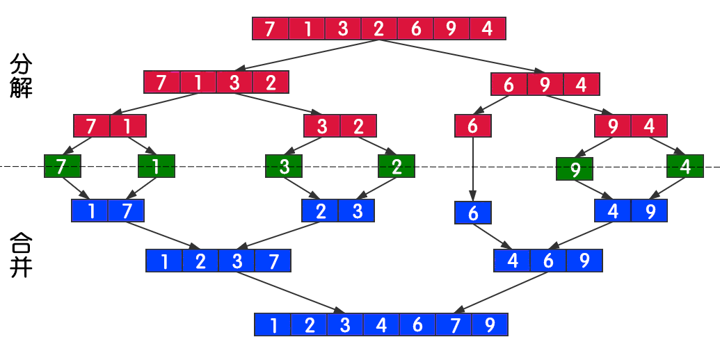
Merge sort is an effective and stable sort algorithm based on merge operation. This algorithm is a very typical application of Divide and Conquer. The ordered subsequences are combined to obtain a completely ordered sequence; That is, each subsequence is ordered first, and then the subsequence segments are ordered. If two ordered tables are merged into one, it is called two-way merging.

2. Steps

Basic steps of merging:

① The application space is the sum of two sorted sequences, and the space is used to store the merged sequences;
② Set two pointers, and the initial position is the starting position of the two sorted sequences respectively;
③ Compare the elements pointed to by the two pointers, select the relatively small element, put it into the merge space, and move the pointer to the next position;
④ Repeat step ③ until a pointer reaches the end of the sequence;
⑤ Copy all the remaining elements of another sequence directly to the end of the merged sequence.

Steps for merging and sorting:

① Decomposition: divide the list smaller and smaller until it is divided into an element. Termination condition: an element is ordered.
② Merge: merge two sequence tables continuously. The list becomes larger and larger until all sequences are merged.

3. Animation demonstration

4. Code implementation

def merge(arr, low, mid, high):
    # low and high are the first and last position indexes of the whole array, and mid is the intermediate position index
    # i and j are pointers, and the initial positions are the starting positions of two ordered sequences respectively
    # ltmp is used to store the merged sequence
    i = low
    j = mid+1
    ltmp = []
    while i <= mid and j <= high:  # As long as there are a few on the left and right
        if arr[i] < arr[j]:        # When the number on the left is less than the number on the right
            ltmp.append(arr[i])    # Store the number on the left in ltmp
            i += 1                 # The left pointer moves one bit to the right
        else:                      # When the number on the right is less than the number on the left
            ltmp.append(arr[j])    # Store the number on the right in ltmp
            j += 1                 # The pointer on the right moves one bit to the right
    # After the above while statement is executed, there are no numbers on the left or right
    while i <= mid:                # When there are still numbers on the left
        ltmp.append(arr[i])        # Save all the remaining numbers on the left into ltmp
        i += 1
    while j <= high:               # When there are still numbers on the right
        ltmp.append(arr[j])        # Save all the remaining numbers on the right into ltmp
        j += 1
    arr[low:high+1] = ltmp         # Write the sorted array back to the original array


def merge_sort(arr, low, high):       # low and high are the first and last position indexes of the entire array
    if low < high:                    # There are at least two elements
        mid = (low + high) // 2
        merge_sort(arr, low, mid)     # Decompose the left recursion
        merge_sort(arr, mid+1, high)  # Decompose the right recursion
        merge(arr, low, mid, high)    # Merge

5. Specific examples

def merge(arr, low, mid, high):
    # low and high are the first and last position indexes of the whole array, and mid is the intermediate position index
    # i and j are pointers, and the initial positions are the starting positions of two ordered sequences respectively
    # ltmp is used to store the merged sequence
    i = low
    j = mid+1
    ltmp = []
    while i <= mid and j <= high:  # As long as there are a few on the left and right
        if arr[i] < arr[j]:        # When the number on the left is less than the number on the right
            ltmp.append(arr[i])    # Store the number on the left in ltmp
            i += 1                 # The left pointer moves one bit to the right
        else:                      # When the number on the right is less than the number on the left
            ltmp.append(arr[j])    # Store the number on the right in ltmp
            j += 1                 # The pointer on the right moves one bit to the right
    # After the above while statement is executed, there are no numbers on the left or right
    while i <= mid:                # When there are still numbers on the left
        ltmp.append(arr[i])        # Save all the remaining numbers on the left into ltmp
        i += 1
    while j <= high:               # When there are still numbers on the right
        ltmp.append(arr[j])        # Save all the remaining numbers on the right into ltmp
        j += 1
    arr[low:high+1] = ltmp         # Write the sorted array back to the original array


def merge_sort(arr, low, high):       # low and high are the first and last position indexes of the entire array
    if low < high:                    # There are at least two elements
        mid = (low + high) // 2
        merge_sort(arr, low, mid)     # Decompose the left recursion
        merge_sort(arr, mid+1, high)  # Decompose the right recursion
        merge(arr, low, mid, high)    # Merge
        print(arr)                    # Print once per merge


arr = [7, 1, 3, 2, 6, 9, 4]
merge_sort(arr, 0, len(arr)-1)

[1, 7, 3, 2, 6, 9, 4]
[1, 7, 2, 3, 6, 9, 4]
[1, 2, 3, 7, 6, 9, 4]
[1, 2, 3, 7, 6, 9, 4]
[1, 2, 3, 7, 4, 6, 9]
[1, 2, 3, 4, 6, 7, 9]

Here is an anti crawler text, please ignore it.
This article was originally launched in CSDN，author TRHX•Bob.
Blog home page: https://itrhx.blog.csdn.net/
Link to this article: https://itrhx.blog.csdn.net/article/details/109251836
 No reprint without authorization! Malicious reprint, bear the consequences! Respect originality and stay away from plagiarism!

6, Quick Sort

1. Principle

Quick sort is an improvement of bubble sort. As the name suggests, quick sorting is fast and efficient! It is one of the fastest sorting algorithms to process big data. Its basic idea is to divide the data to be sorted into two independent parts through one-time sorting. All the data in one part is smaller than all the data in the other part, and then quickly sort the two parts of data according to this method. The whole sorting process can be recursive, so that the whole data becomes an ordered sequence.

2. Steps

① Select an element from the sequence, which is called "reference value";
② Reorder the sequence. All elements smaller than the benchmark value are placed on the left of the benchmark value, and those larger than the benchmark value are placed on the right of the benchmark value (the same number can be on either side). After the partition exits, the reference value is in the middle of the sequence. This is called a partition operation, which can also be called a homing operation. The process of homing operation is shown in the following figure;
③ Recursively sort the subsequence less than the reference value element and the subsequence greater than the reference value element according to steps ① and ②.

3. Animation demonstration

4. Code implementation

def partition(arr, left, right):
    # Return operation, left and right are the position indexes on the left and right of the array respectively
    tmp = arr[left]
    while left < right:
        while left < right and arr[right] >= tmp:  # Find a number smaller than tmp from the right. If it is larger than tmp, move the pointer
            right -= 1                             # Move the pointer one position to the left
        arr[left] = arr[right]                     # Write the value on the right to the empty space on the left
        while left < right and arr[left] <= tmp:   # Find a number larger than tmp from the left. If it is smaller than tmp, move the pointer
            left += 1                              # Move the pointer one position to the right
        arr[right] = arr[left]                     # Write the value on the left to the empty space on the right
    arr[left] = tmp                                # Put tmp back
    return left                   # Both left and right can be returned to facilitate the subsequent recursive operation to sort the left and right parts


def quick_sort(arr, left, right):          # Quick sort
    if left < right:
        mid = partition(arr, left, right)
        quick_sort(arr, left, mid-1)       # Homing the left half
        quick_sort(arr, mid+1, right)      # Return the right half
    return arr

5. Specific examples

def partition(arr, left, right):
    # Return operation, left and right are the position indexes on the left and right of the array respectively
    tmp = arr[left]
    while left < right:
        while left < right and arr[right] >= tmp:  # Find a number smaller than tmp from the right. If it is larger than tmp, move the pointer
            right -= 1                             # Move the pointer one position to the left
        arr[left] = arr[right]                     # Write the value on the right to the empty space on the left
        while left < right and arr[left] <= tmp:   # Find a number larger than tmp from the left. If it is smaller than tmp, move the pointer
            left += 1                              # Move the pointer one position to the right
        arr[right] = arr[left]                     # Write the value on the left to the empty space on the right
    arr[left] = tmp                                # Put tmp back
    return left                   # Both left and right can be returned to facilitate the subsequent recursive operation to sort the left and right parts


def quick_sort(arr, left, right):
    if left < right:
        mid = partition(arr, left, right)
        print(arr)                         # Print once after each homing
        quick_sort(arr, left, mid-1)       # Homing the left half
        quick_sort(arr, mid+1, right)      # Return the right half


arr = [5, 7, 4, 6, 3, 1, 2, 9, 8]
quick_sort(arr, 0, len(arr)-1)

[2, 1, 4, 3, 5, 6, 7, 9, 8]
[1, 2, 4, 3, 5, 6, 7, 9, 8]
[1, 2, 3, 4, 5, 6, 7, 9, 8]
[1, 2, 3, 4, 5, 6, 7, 9, 8]
[1, 2, 3, 4, 5, 6, 7, 9, 8]
[1, 2, 3, 4, 5, 6, 7, 8, 9]

7, Heap Sort

1. Principle

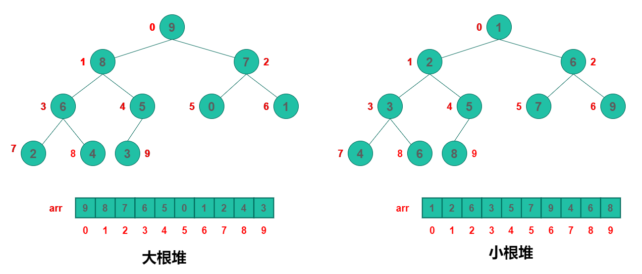
Heap sort is a sort algorithm designed by using heap data structure. Heap is a structure similar to a complete binary tree and satisfies the nature of heap: that is, the key value or index of a child node is always less than (or greater than) its parent node.

Heap: a special complete binary tree structure
Large root heap: a complete binary tree that satisfies that any node is larger than its child node
Small root heap: a complete binary tree, satisfying that any node is smaller than its child node

2. Steps

① Build heap: build the sequence to be sorted into a heap H[0... n-1], starting from the last non leaf node, adjusting from left to right and from bottom to top. Select large top stack or small top stack according to ascending or descending requirements;
② The heap top element at this time is the maximum or minimum element;
③ Exchange the top and tail elements of the heap, adjust the heap and re order the heap;
④ At this time, the top element is the second largest element;
⑤ Repeat the above steps until the reactor becomes empty.

3. Animation demonstration

Push sort after heap Construction:

4. Code implementation

def sift(arr, low, high):
    """
    :param li: list
    :param low: Root node location of the heap
    :param high: The position of the last element of the heap
    """
    i = low                 # i initially points to the root node
    j = 2 * i + 1           # j started as a left child
    tmp = arr[low]          # Store the top of the pile
    while j <= high:        # As long as there are several j positions
        if j + 1 <= high and arr[j+1] > arr[j]:   # If the right child has and is older
            j = j + 1       # j points to the right child
        if arr[j] > tmp:
            arr[i] = arr[j]
            i = j           # Look down one floor
            j = 2 * i + 1
        else:               # tmp is bigger. Put tmp in the position of i
            arr[i] = tmp    # Put tmp in a leadership position at a certain level
            break
    else:
        arr[i] = tmp        # Put tmp on leaf node


def heap_sort(arr):
    n = len(arr)
    for i in range((n-2)//2, - 1, - 1): # I indicates the subscript of the root of the adjusted part during heap building
        sift(arr, i, n-1)
    # Completion of reactor building
    for i in range(n-1, -1, -1):        # i points to the last element of the current heap
        arr[0], arr[i] = arr[i], arr[0]
        sift(arr, 0, i - 1)             # i-1 is the new high
    return arr

5. Specific examples

def sift(arr, low, high):
    """
    :param li: list
    :param low: Root node location of the heap
    :param high: The position of the last element of the heap
    """
    i = low                 # i initially points to the root node
    j = 2 * i + 1           # j started as a left child
    tmp = arr[low]          # Store the top of the pile
    while j <= high:        # As long as there are several j positions
        if j + 1 <= high and arr[j+1] > arr[j]:   # If the right child has and is older
            j = j + 1       # j points to the right child
        if arr[j] > tmp:
            arr[i] = arr[j]
            i = j           # Look down one floor
            j = 2 * i + 1
        else:               # tmp is bigger. Put tmp in the position of i
            arr[i] = tmp    # Put tmp in a leadership position at a certain level
            break
    else:
        arr[i] = tmp        # Put tmp on leaf node


def heap_sort(arr):
    n = len(arr)
    print('Reactor building process:')
    print(arr)
    for i in range((n-2)//2, - 1, - 1): # I indicates the subscript of the root of the adjusted part during heap building
        sift(arr, i, n-1)
        print(arr)
    # Completion of reactor building
    print('Heap sort process:')
    print(arr)
    for i in range(n-1, -1, -1):        # i points to the last element of the current heap
        arr[0], arr[i] = arr[i], arr[0]
        sift(arr, 0, i - 1)             # i-1 is the new high
        print(arr)


arr = [2, 7, 26, 25, 19, 17, 1, 90, 3, 36]
heap_sort(arr)

Reactor building process:
[2, 7, 26, 25, 19, 17, 1, 90, 3, 36]
[2, 7, 26, 25, 36, 17, 1, 90, 3, 19]
[2, 7, 26, 90, 36, 17, 1, 25, 3, 19]
[2, 7, 26, 90, 36, 17, 1, 25, 3, 19]
[2, 90, 26, 25, 36, 17, 1, 7, 3, 19]
[90, 36, 26, 25, 19, 17, 1, 7, 3, 2]
Heap sort process:
[90, 36, 26, 25, 19, 17, 1, 7, 3, 2]
[36, 25, 26, 7, 19, 17, 1, 2, 3, 90]
[26, 25, 17, 7, 19, 3, 1, 2, 36, 90]
[25, 19, 17, 7, 2, 3, 1, 26, 36, 90]
[19, 7, 17, 1, 2, 3, 25, 26, 36, 90]
[17, 7, 3, 1, 2, 19, 25, 26, 36, 90]
[7, 2, 3, 1, 17, 19, 25, 26, 36, 90]
[3, 2, 1, 7, 17, 19, 25, 26, 36, 90]
[2, 1, 3, 7, 17, 19, 25, 26, 36, 90]
[1, 2, 3, 7, 17, 19, 25, 26, 36, 90]
[1, 2, 3, 7, 17, 19, 25, 26, 36, 90]

8, Counting Sort

1. Principle

Counting sorting is a non comparison based sorting algorithm. Its advantage is that when sorting integers in a certain range, its complexity is Ο (n+k), where k is the range of integers, faster than any comparison sorting algorithm. Counting sorting is a method of sacrificing space for time. The core of counting sorting is to convert the input data values into keys and store them in the additional array space. As a sort with linear time complexity, count sort requires that the input data must be integers with a certain range.

2. Steps

① Find the maximum value k in the list to be sorted, and open up a count list with a length of k+1. The values in the count list are 0.
② Traverse the list to be sorted. If the traversed element value is i, the value of index i in the count list is increased by 1.
③ Traverse the complete list to be sorted, count the value J of index i in the list, indicating that the number of i is j, and count the number of each value in the list to be sorted.
④ Create a new list (or empty the original list and add it to the original list), traverse the count list and add j i's to the new list in turn. The new list is the ordered list. The data size in the list to be sorted is not compared in the whole process.

3. Animation demonstration

4. Code implementation

def count_sort(arr):
    if len(arr) < 2:                       # If the array length is less than 2, it is returned directly
        return arr
    max_num = max(arr)
    count = [0 for _ in range(max_num+1)]  # Open up a count list
    for val in arr:
        count[val] += 1
    arr.clear()                        # Empty original array
    for ind, val in enumerate(count):  # Traversal value and subscript (number of values)
        for i in range(val):
            arr.append(ind)
    return arr

5. Specific examples

def count_sort(arr):
    if len(arr) < 2:                       # If the array length is less than 2, it is returned directly
        return arr
    max_num = max(arr)
    count = [0 for _ in range(max_num+1)]  # Open up a count list
    for val in arr:
        count[val] += 1
    arr.clear()                        # Empty original array
    for ind, val in enumerate(count):  # Traversal value and subscript (number of values)
        for i in range(val):
            arr.append(ind)
    return arr


arr = [2, 3, 8, 7, 1, 2, 2, 2, 7, 3, 9, 8, 2, 1, 4, 2, 4, 6, 9, 2]
sorted_arr = count_sort(arr)
print(sorted_arr)

[1, 1, 2, 2, 2, 2, 2, 2, 2, 3, 3, 4, 4, 6, 7, 7, 8, 8, 9, 9]

9, Bucket Sort

1. Principle

Bucket sorting is also called box sorting. The working principle is to divide the array into a limited number of buckets. Each bucket is sorted individually (it is possible to use another sorting algorithm or continue to use bucket sorting recursively). Bucket sorting is an inductive result of pigeon nest sorting.

Bucket sorting is also an upgraded version of counting sorting. It makes use of the mapping relationship of the function. The key to efficiency lies in the determination of the mapping function. In order to make bucket sorting more efficient, we need to do these two things:

Increase the number of barrels as much as possible with sufficient additional space;
The mapping function used can evenly distribute the input N data into K buckets.

At the same time, for the sorting of elements in the bucket, it is very important to choose a comparative sorting algorithm for the performance.

Fastest case: when the input data can be evenly distributed to each bucket;
Slowest case: when the input data is allocated to the same bucket.

2. Steps

① Create a quantitative array as an empty bucket;
② Traverse the sequence and put the elements into the corresponding bucket one by one;
③ Sort each bucket that is not empty;
④ Put the elements back into the original sequence from a bucket that is not empty.

3. Animation demonstration

(the dynamic graph is derived from @ five minute learning algorithm, invasion and deletion)

4. Code implementation

def bucket_sort(arr):
    max_num = max(arr)
    n = len(arr)
    buckets = [[] for _ in range(n)]         # Create bucket
    for var in arr:
        i = min(var // (max_num / / N), n-1) # I indicates the number of buckets var is placed in
        buckets[i].append(var)               # Add var to the bucket
        # Keep the order in the bucket
        for j in range(len(buckets[i])-1, 0, -1):
            if buckets[i][j] < buckets[i][j-1]:
                buckets[i][j], buckets[i][j-1] = buckets[i][j-1], buckets[i][j]
            else:
                break
    sorted_arr = []
    for buc in buckets:
        sorted_arr.extend(buc)
    return sorted_arr

5. Specific examples

def bucket_sort(arr):
    max_num = max(arr)
    n = len(arr)
    buckets = [[] for _ in range(n)]         # Create bucket
    for var in arr:
        i = min(var // (max_num / / N), n-1) # I indicates the number of buckets var is placed in
        buckets[i].append(var)               # Add var to the bucket
        # Keep the order in the bucket
        for j in range(len(buckets[i])-1, 0, -1):
            if buckets[i][j] < buckets[i][j-1]:
                buckets[i][j], buckets[i][j-1] = buckets[i][j-1], buckets[i][j]
            else:
                break
    sorted_arr = []
    for buc in buckets:
        sorted_arr.extend(buc)
    return sorted_arr


arr = [7, 12, 56, 23, 19, 33, 35, 42, 42, 2, 8, 22, 39, 26, 17]
sorted_arr = bucket_sort(arr)
print(sorted_arr)

[2, 7, 8, 12, 17, 19, 22, 23, 26, 33, 35, 39, 42, 42, 56]

10, Radix Sort

1. Principle

Cardinal sorting belongs to distributive sorting. It is a non comparative integer sorting algorithm. Its principle is to cut integers into different numbers according to the number of bits, and then compare them according to each number of bits. Since integers can also express strings (such as names or dates) and floating-point numbers in a specific format, cardinality sorting is not limited to integers.

The three sorting algorithms of cardinality sorting, counting sorting and bucket sorting all use the concept of bucket, but there are obvious differences in the use of bucket:

Cardinality sorting: allocate buckets according to each number of the key value;
Counting and sorting: only one key value is stored in each bucket;
Bucket sorting: each bucket stores a certain range of values.

2. Steps

① Get the maximum number in the array and get the number of bits;
② Start from the lowest order and sort once in sequence;
③ From the lowest order to the highest order, the sequence becomes an ordered sequence.

3. Animation demonstration

4. Code implementation

def radix_sort(li):
    max_num = max(li)      # Maximum 9 - > 1 cycle, 99 - > 2 cycles, 888 - > 3 cycles, 10000 - > 5 cycles
    it = 0
    while 10 ** it <= max_num:
        buckets = [[] for _ in range(10)]
        for var in li:
            # var=987, it=1, 987//10->98, 98%10->8; it=2, 987//100->9, 9%10=9
            digit = (var // 10 * * it)% 10 # take one digit in turn
            buckets[digit].append(var)
        # Completion of barrel separation
        li.clear()
        for buc in buckets:
            li.extend(buc)
        it += 1            # Rewrite the number back to li
    return arr

5. Specific examples

def radix_sort(li):
    max_num = max(li)      # Maximum 9 - > 1 cycle, 99 - > 2 cycles, 888 - > 3 cycles, 10000 - > 5 cycles
    it = 0
    while 10 ** it <= max_num:
        buckets = [[] for _ in range(10)]
        for var in li:
            # var=987, it=1, 987//10->98, 98%10->8; it=2, 987//100->9, 9%10=9
            digit = (var // 10 * * it)% 10 # take one digit in turn
            buckets[digit].append(var)
        # Completion of barrel separation
        li.clear()
        for buc in buckets:
            li.extend(buc)
        it += 1            # Rewrite the number back to li
    return arr


arr = [3221, 1, 10, 9680, 577, 9420, 7, 5622, 4793, 2030, 3138, 82, 2599, 743, 4127]
sorted_arr = radix_sort(arr)
print(sorted_arr)

[1, 7, 10, 82, 577, 743, 2030, 2599, 3138, 3221, 4127, 4793, 5622, 9420, 9680]

This article is composed of one article multi posting platform ArtiPub Auto publish

Added by Poolie on Mon, 17 Jan 2022 13:30:01 +0200

Programming VIP

Python implements ten classic sorting algorithms artipub

Sorting algorithm classification

1, Bubble Sort

1. Principle

2. Steps

3. Animation demonstration

4. Code implementation

5. Specific examples

2, Selection Sort

1. Principle

2. Steps

3. Animation demonstration

4. Code implementation

5. Specific examples

3, Insertion Sort

1. Principle

2. Steps

3. Animation demonstration

4. Code implementation

5. Specific examples

4, Shell Sort

1. Principle

2. Steps

3. Animation demonstration

4. Code implementation

5. Specific examples

5, Merge Sort

1. Principle

2. Steps

3. Animation demonstration

4. Code implementation

5. Specific examples

6, Quick Sort

1. Principle

2. Steps

3. Animation demonstration

4. Code implementation

5. Specific examples

7, Heap Sort

1. Principle

2. Steps

3. Animation demonstration

4. Code implementation

5. Specific examples

8, Counting Sort

1. Principle

2. Steps

3. Animation demonstration

4. Code implementation

5. Specific examples

9, Bucket Sort

1. Principle

2. Steps

3. Animation demonstration

4. Code implementation

5. Specific examples

10, Radix Sort

1. Principle

2. Steps

3. Animation demonstration

4. Code implementation

5. Specific examples

Popular Keywords