Time series (or dynamic series) refers to the sequence of the values of the same statistical index according to their occurrence time. The main purpose of time series analysis is to predict the future based on the existing historical data. In this paper, we will share how to use historical stock data for basic time series analysis (hereinafter referred to as time series analysis). First, we will create a static prediction model to test the validity of the model, and then share some important tools for time series analysis.

Before creating the model, we first briefly understand some basic parameters of time series, such as moving average, trend, seasonality and so on.

get data

We will use MRF's "price adjustment" over the past five years, and use pandas_data reader to get the data needed from Yahoo Finance and Economics. First we import the required libraries:

import pandas as pd
import pandas_datareader as web
import matplotlib.pyplot as plt
import numpy as np

Now we use data reader to get data, mainly from January 1, 2012 to December 21, 2017. Of course, you can only adjust the closing price, because this is the most relevant price, which is applied in all financial analysis.

stock = web.DataReader('MRF.BO','yahoo', start = "01-01-2012", end="31-12-2017")
stock = stock.dropna(how='any')

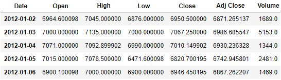
We can use the head() function to check the data.

stock.head()

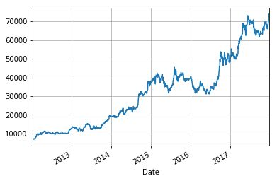
We can use the imported matplotlib library to plot the adjusted price again over time.

stock['Adj Close'].plot(grid = True)

Calculating and mapping daily earnings

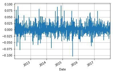
Using the time series, we can calculate the daily income which changes with time and draw the income change chart. We will calculate daily earnings from the adjusted closing price of stock s and store them in the same data frame as "ret".

stock['ret'] = stock['Adj Close'].pct_change()
stock['ret'].plot(grid=True)

Moving average

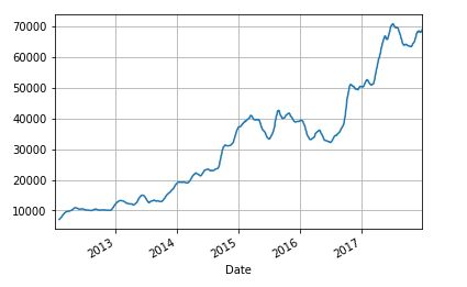
As with earnings, we can calculate and plot moving averages that adjust closing prices. Moving average is a very important index widely used in technical analysis. For the purpose of illustration, we only calculate the 20-day moving average as an example.

stock['20d'] = stock['Adj Close'].rolling(window=20, center=False).mean()
stock['20d'].plot(grid=True)

Before building a model to predict, let's quickly look at the trend and seasonality in time series.

Trends and Seasonality

Simply put, trends represent the overall direction of time series over a period of time. Trend and trend analysis are also widely used in technical analysis. If there are regular patterns in the time series, we say that the data are seasonal. Seasonality in time series can affect the results of prediction models, so it should not be taken lightly.

If you are still confused in the world of programming, you can join our Python Learning button qun: 784758214 to see how our predecessors learned. Exchange of experience. From basic Python script to web development, crawler, django, data mining, zero-base to actual project data are sorted out. To every Python buddy! Share some learning methods and small details that need attention. Click to join us. python learner gathering place

Forecast

We will discuss a simple linear analysis model, assuming that the time series is static and not seasonal. That is to say, we assume that the time series has a linear trend. The model can be expressed as:

Forecast (t) = a + b X t

Here "a" is the intercept of time series on the Y axis, and "b" is the slope. Now let's look at the calculations of a and B. We consider the value D (t) of time series in time interval "t".

In this equation, "n" is the sample size. We can validate our model by calculating the predicted value of D (t) and comparing the predicted value with the observed value. We can calculate the average error, that is, the average value of the difference between the predicted D (t) value and the actual D (t) value.

In our stock data, D (t) is the adjusted closing price of MRF. We now use Python to calculate a,b, predictions and their error values.

#Populates the time period number in stock under head t
stock['t'] = range (1,len(stock)+1)

#Computes t squared, tXD(t) and n
stock['sqr t']=stock['t']**2
stock['tXD']=stock['t']*stock['Adj Close']
n=len(stock)

#Computes slope and intercept
slope = (n*stock['tXD'].sum() - stock['t'].sum()*stock['Adj Close'].sum())/(n*stock['sqr t'].sum() - (stock['t'].sum())**2)
intercept = (stock['Adj Close'].sum()*stock['sqr t'].sum() - stock['t'].sum()*stock['tXD'].sum())/(n*stock['sqr t'].sum() - (stock['t'].sum())**2)
print ('The slope of the linear trend (b) is: ', slope)
print ('The intercept (a) is: ', intercept)

The above code gives the following output:

The slope of the linear trend (b) is: 41.2816591061

The intercept (a) is: 1272.6557803

We can now verify the validity of the model by calculating the predicted value and the average error.

#Computes the forecasted values
stock['forecast'] = intercept + slope*stock['t']

#Computes the error
stock['error'] = stock['Adj Close'] - stock['forecast']
mean_error=stock['error'].mean()
print ('The mean error is: ', mean_error)

The average error of the output is as follows:

The mean error is: 1.0813935108094419e-10

From the average error value, we can see that the value given by our model is very close to the actual value. So the data are not affected by any seasonal factors.

Next, we discuss some useful tools for analyzing time series data, which are very helpful for financial traders in designing and pre-testing trading strategies.

Traders often have to process a large amount of historical data and analyze the data according to these time series. Here we focus on how to deal with the date and frequency of time series, as well as indexing, slicing and other operations. datetime libraries are mainly used.

We first import the datetime library into the program.

#Importing the required modules

from datetime import datetime
from datetime import timedelta

Basic tools for dealing with dates and times

First, save the current date and time in the variable "current_time", and execute the code as follows:

#Printing the current date and time

current_time = datetime.now()
current_time
Output: datetime.datetime(2018, 2, 14, 9, 52, 20, 625404)

We can use datetime to calculate the difference between the two dates.

#Calculating the difference between two dates (14/02/2018 and 01/01/2018 09:15AM)

delta = datetime(2018,2,14)-datetime(2018,1,1,9,15)
delta
Output: datetime.timedelta(43, 53100)

Use the following code to convert the output to "days" or "seconds":

#Converting the output to days

delta.days
Output: 43

#Converting the output to seconds

delta.seconds
Output: 53100

If we want to change the date, we can use the timedelta module imported earlier.

#Shift a date using timedelta

my_date = datetime(2018,2,10)

#Shift the date by 10 days

my_date + timedelta(10)
Output: datetime.datetime(2018, 2, 20, 0, 0)

We can also use the multiplication of the timedelta function.

#Using multiples of timedelta function

my_date - 2*timedelta(10)
Output: datetime.datetime(2018, 1, 21, 0, 0)

We saw the "datetime" and "time delta" data types of the datetime module earlier. We briefly describe the main data types used in time series analysis:

data type

describe

Date

Keep calendar dates (year, month, day) in the Gregorian calendar

Time

Save time as hours, minutes, seconds, and microseconds

Datetime

Save date and time data types

Timedelta

Save the difference between two datetime values

Conversion between strings and datetime

We can convert the datetime format to a string and save it as a string variable. Conversely, you can convert a string representing a date to a datetime data type.

#Converting datetime to string

my_date1 = datetime(2018,2,14)
str(my_date1)
Output: '2018-02-14 00:00:00'

We can use the strptime function to convert strings to datetime.

#Converting a string to datetime

datestr = '2018-02-14'
datetime.strptime(datestr, '%Y-%m-%d')
Output: datetime.datetime(2018, 2, 14, 0, 0)

You can also use Pandas to process dates. Let's import Pandas first.

#Importing pandas

import pandas as pd

In Pandas, "to_datetime" is used to convert date strings to date data types.

#Using pandas to parse dates

datestrs = ['1/14/2018', '2/14/2018']
pd.to_datetime(datestrs)
Output: DatetimeIndex(['2018-01-14', '2018-02-14'], dtype='datetime64[ns]', freq=None)

In Pandas, the missing time or NA value in time is expressed as NaT.

Index and Slice of Time Series

In order to better understand the multiple operations in time series, we use random numbers to create a time series.

#Creating a time series with random numbers

import numpy as np
from random import random
dates = [datetime(2011, 1, 2), datetime(2011, 1, 5), datetime(2011, 1, 7), datetime(2011, 1, 8), datetime(2011, 1, 10), datetime(2011, 1, 12)]
ts = pd.Series(np.random.randn(6), index=dates)
ts

Output:
2011-01-02   0.888329
2011-01-05  -0.152267
2011-01-07   0.854689
2011-01-08   0.680432
2011-01-10   0.123229
2011-01-12  -1.503613
dtype: float64

With the index we show, the elements of the time series can be invoked as any other Pandas sequence.

ts ['01/02/2011'] or ts ['20110102'] will give the same output of 0.888329

The slicing operation is the same as that of other Pandas sequences.

Repeated Index in Time Series

Sometimes your time series contains duplicate indexes. Look at the following time series:

#Slicing the time series

ts[datetime(2011,1,7):]
Output:
2011-01-07 0.854689
2011-01-08 0.680432
2011-01-10 0.123229
2011-01-12 -1.503613
dtype: float64

In the above time series, we can see that "2018-01-02" repeated three times. We can check this with the "is_unique" attribute of the index function.

dup_ts.index.is_unique
Output: False

You can use the groupby feature set to have records with the same index.

grouped=dup_ts.groupby(level=0)

We can now use the average, count, sum and so on of these records according to our own needs.

grouped.mean()
Output:
2018-01-01 -0.471411
2018-01-02 -0.013973
2018-01-03 -0.611886
dtype: float64

grouped.count()
Output:
2018-01-01 1
2018-01-02 3
2018-01-03 1
dtype: int64

grouped.sum()
Output:
2018-01-01 -0.471411
2018-01-02 -0.041920
2018-01-03 -0.611886
dtype: float64

Data displacement

We can use shift function to transfer the index of time series.

#Shifting the time series
ts.shift(2)
Output:
2011-01-02 NaN
2011-01-05 NaN
2011-01-07 0.888329
2011-01-08 -0.152267
2011-01-10 0.854689
2011-01-12 0.680432
dtype: float64
 What I don't know in the process of learning can be added to me?
python learning communication deduction qun, 784758214
 There are good learning video tutorials, development tools and e-books in the group.
Share with you the current talent needs of python enterprises and how to learn python from zero foundation, and what to learn

summary

In this paper, we briefly discuss some properties of time series and how to calculate them with Python. At the same time, a simple linear model is used to predict time series. Finally, some basic functions used in time series analysis are shared, such as converting dates from one format to another.