Preface

Previously, I have talked about the path of python machine learning. This time, Luo Luopan takes you to complete a machine learning project of Chinese text sentiment analysis. Today's process is as follows:

Data Situation and Processing

Data situation

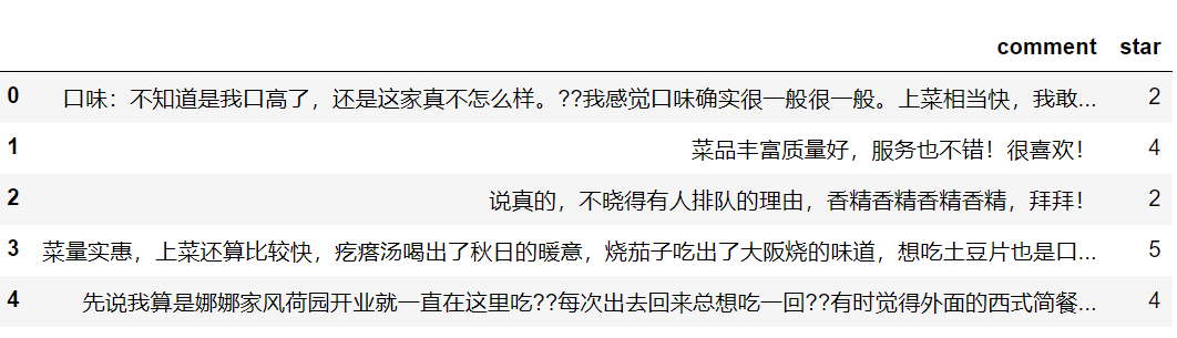
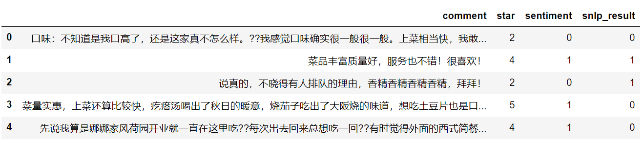
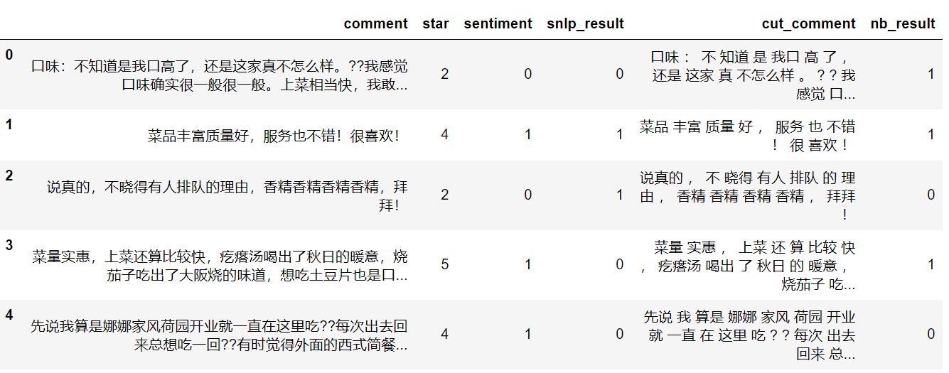
The data here are for the comments of the public (provided by Mr. Wang Shuyi), mainly the comments and scores. Let's first read in the data and see what happens to the data.

import numpy as np
import pandas as pd
data = pd.read_csv('data1.csv')
data.head()

Emotion partition

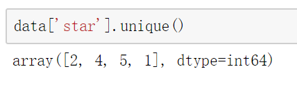
Look at the unique value for the star field and score 1, 2, 4, 5.

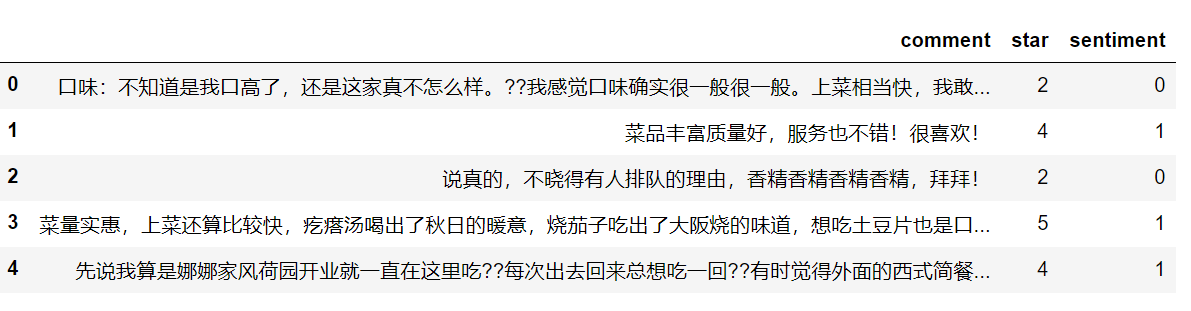
Emotional analysis of Chinese text belongs to our classification problem (that is, negative and positive). Here is the score. Then we design the code to make the score less than 3 negative (0), and more than 3 positive (1).

Define a function and then use the apply method to get a new column (knowledge points in data analysis)

def make_label(star):
    if star > 3:
        return 1
    else:
        return 0
    
data['sentiment'] = data.star.apply(make_label)

Toolkit (snownlp)

First of all, we don't need machine learning methods. We use a third library (snownlp), which can directly analyze the text emotionally (remember to install), and the method is simple. The return is the probability of motivation.

from snownlp import SnowNLP

text1 = 'This is a good thing.'
text2 = 'It's rubbish.'

s1 = SnowNLP(text1)
s2 = SnowNLP(text2)

print(s1.sentiments,s2.sentiments)
# result 0.8623218777387431 0.21406279508712744

In this way, we define more than 0.6, that is, positive, the same way, we can get results.

def snow_result(comemnt):
    s = SnowNLP(comemnt)
    if s.sentiments >= 0.6:
        return 1
    else:
        return 0
    
data['snlp_result'] = data.comment.apply(snow_result)

The results of the first five lines above look bad (2 out of 5 are right), so how many are right? We can compare the results with the sentiment field, and I count them equally, so that by dividing the total sample, we can see the approximate accuracy.

counts = 0
for i in range(len(data)):
    if data.iloc[i,2] == data.iloc[i,3]:
        counts+=1

print(counts/len(data))
# result 0.763

Naive Bayes

The result of using the third library method is not particularly ideal (0.763), and this method has a big disadvantage: poor pertinence.

What do you mean? We all know that in different scenarios, language expression is different. For example, this is useful in product evaluation and may not be applicable in blog comments.

So we need to train our models for this scenario. This paper will use sklearn to implement naive Bayesian model (the principle will be explained later). Slarn transcripts are sent to you first (the following is the HD download address).

Probably the process is as follows:

• Import data
• Segmentation data
• Data preprocessing
• Training model
• test model

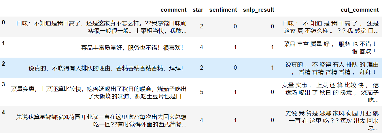
jieba participle

First of all, we participle the comment data. Why participle? Chinese is different from English, for example, i love python, which is partitioned by spaces; we are different in Chinese, for example: I like programming, we need to divide it into me / like / programming (separated by spaces), which is mainly for preparing the latter word vector.

import jieba

def chinese_word_cut(mytext):
    return " ".join(jieba.cut(mytext))

data['cut_comment'] = data.comment.apply(chinese_word_cut)

Partition of data sets

Classification problems need x (features) and Y (label). The comment after participle here is x and the emotion is y. According to the ratio of 8:2, it is divided into training set and test set.

X = data['cut_comment']
y = data.sentiment

from sklearn.model_selection import train_test_split

X_train, X_test, y_train, y_test = train_test_split(X, y, test_size=0.2, random_state=22)

Word Vector (Data Processing)

Computers can't recognize words, they can only recognize numbers. The simplest way to deal with the text is the word vector. What is a word vector? Let's illustrate it with a case study. Here's our text.

I love the dog
I hate the dog 

Word vector processing is like this:

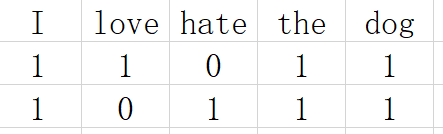
Simply put, the word vector is that we arrange the words that appear in the whole text one by one, and then map each row of data to these columns. It appears as 1, and it does not appear as 0. In this way, the text data is converted into a 01 sparse matrix (which is also the reason for the Chinese word segmentation above, such a word is a column).

Fortunately, sklearn s directly have such a method for us to use. The parameters commonly used in CountVectorizer method are:

• max_df: Keywords (too trivial) that appear in documents that exceed this ratio are removed.
• min_df: Keywords (too unique) that appear in documents below this number are removed.
• token_pattern: Numbers and punctuation are removed mainly through regularization.
• Sto_words: Setting up a stop list, such words will not be counted out (mostly virtual words, articles, etc.). We need a list structure, so the code defines a function to handle the stop list.

from sklearn.feature_extraction.text import CountVectorizer

def get_custom_stopwords(stop_words_file):
    with open(stop_words_file) as f:
        stopwords = f.read()
    stopwords_list = stopwords.split('\n')
    custom_stopwords_list = [i for i in stopwords_list]
    return custom_stopwords_list

stop_words_file = 'Terminology of Hatou University of Technology.txt'
stopwords = get_custom_stopwords(stop_words_file)

vect = CountVectorizer(max_df = 0.8, 
                       min_df = 3, 
                       token_pattern=u'(?u)\\b[^\\d\\W]\\w+\\b', 
                       stop_words=frozenset(stopwords))

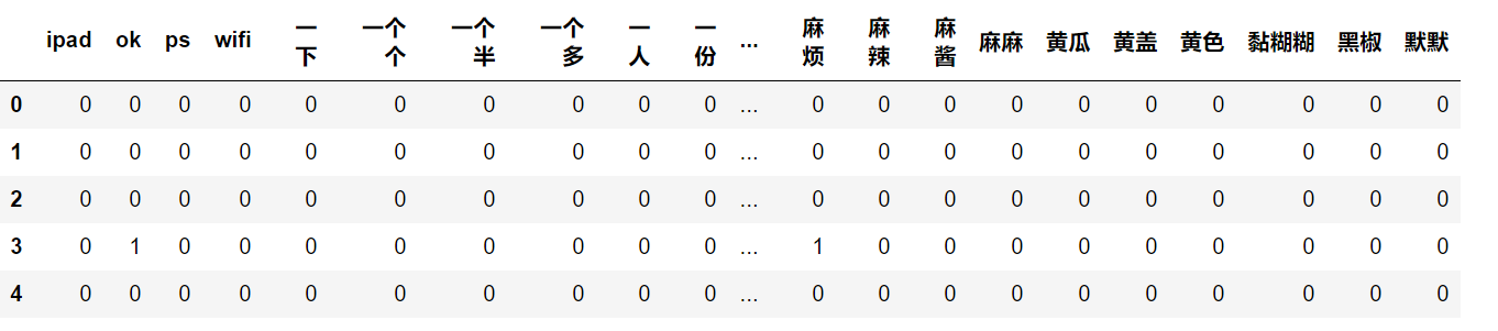
If you want to see what the bottom data is, you can see it through the following code.

test = pd.DataFrame(vect.fit_transform(X_train).toarray(), columns=vect.get_feature_names())
test.head()

Training model

The training model is very simple, using the naive Bayesian algorithm, the result is 0.899, much better than the previous snownlp.

from sklearn.naive_bayes import MultinomialNB
nb = MultinomialNB()

X_train_vect = vect.fit_transform(X_train)
nb.fit(X_train_vect, y_train)
train_score = nb.score(X_train_vect, y_train)
print(train_score)

# result 0.899375

test data

Of course, we need test data to verify the accuracy, the result is 0.8275, the accuracy is still good.

X_test_vect = vect.transform(X_test)
print(nb.score(X_test_vect, y_test))

# result 0.8275

Of course, we can also put the results into data data data:

X_vec = vect.transform(X)
nb_result = nb.predict(X_vec)
data['nb_result'] = nb_result

Discussions and shortcomings

• Less sample size
• The model does not adjust parameters
• No cross validation

Today's interaction

Code download: https://github.com/panluoluo/crawler-analysis Download the complete data and code.

Message punching: Tell me about the comments. The public responded back-stage, joined the card learning group, and worked together in 2019.