This article mainly records the process of using machine learning to solve the problems I encounter.

catalogue

1, Problem description

2, Data processing

2.1 treatment of missing values

2.2 abnormal value handling

2.3 characteristic Engineering

3, Dimensionality reduction

4, Model establishment

5, Model training

1, Problem description

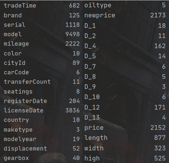
First of all, there are two questions in the data set of data 1 and data 2. We need to give a brief description of the data set of data 1 and data 2. Both data sets contain 36 columns of variables, and the variable fields are shown in the figure below:

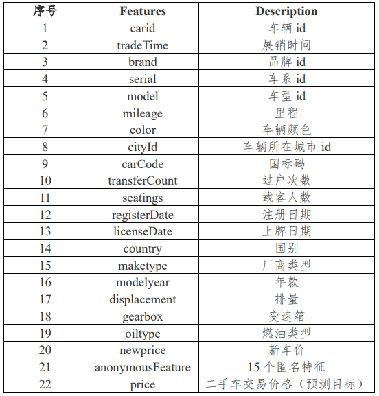
There are 15 anonymous variables. The difference between datasets data1 and data2 is that the price variable of data1 has data, while the price of data2 needs to be filled in. In other words, the topic requires us to use data1 data set to establish a model and use the established model to predict the used car price in data2.

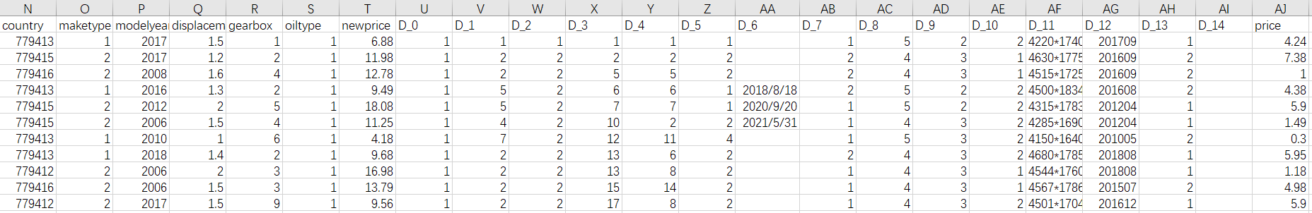
Part of data1 data is as follows:

Part of data2 data is as follows:

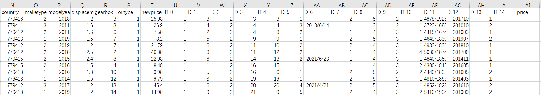
It can be seen that I numbered 15 anonymous variables from D_0 to D_14. There is no data for the price variable in data2, which requires us to predict. Another thing to mention is that in fact, the variable D_14 has data, but it has too many missing values. The screenshot just shows that it has no data. Next, start to solve it step by step.

2, Data processing

2.1 treatment of missing values

The first thing is to check the missing value of the data and deal with it. We first read the data into training set and test set respectively, and then merge the two data sets:

Train = pd.read_csv('E:\\data1.csv', delimiter=',')  # Training set
Test = pd.read_csv('E:\\data2.csv', delimiter=',')  # Test set
print('Train shape: ', Train.shape)
print('Test shape: ', Test.shape)
Combine = pd.concat([Train, Test])  # Merge test set and training set
print('Combine shape: ', Combine.shape)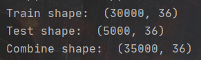

The above figure shows the data dimensions of training set and test set, as well as the combined dimensions. Next, use ISNA () The sum () function looks at the missing values of the columns in the dataset.

print(Combine.isna().sum())  # Number of missing values in each column of statistical data set

In order to more intuitively see the actual situation of the data, I rank the variables with missing values from high to low according to the number of missing values, and visualize them:

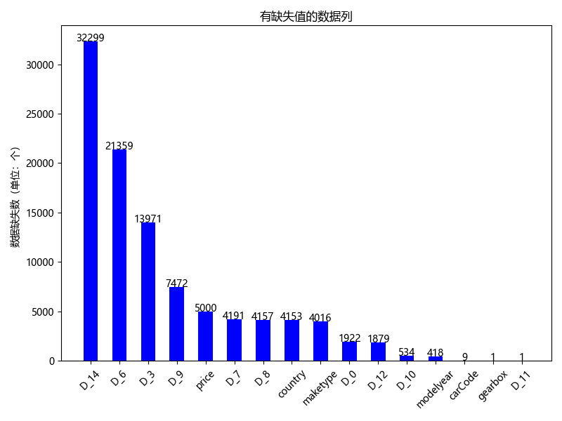
It can be seen from the above figure that there are 16 columns of variables with missing values, of which 5000 missing values of price variable are for us to predict, so no additional processing is required. For D_14,D_6 and D_3. We can see that there are too many missing values, which is not helpful to the training of the model, or even noise, so we delete them. For D_9,D_7,D_8. In order to avoid having a great impact on the overall data distribution of the country and maketype columns, we fill them with the data of the previous cell with missing value. If the previous cell is also missing value, we fill them with the mode of the data column. And for D_0,D_12,D_10,modelyear,carCode,gearbox,D_11 these columns of data have relatively few missing values, so we fill them with the modes of their corresponding columns respectively.

If the mode is filled, the following code can be used for operation, which is convenient and fast:

Combine = Combine.fillna(Combine.mode().iloc[0, :])  # Fill with the data that appears most in each column.

2.2 abnormal value handling

First, you can use combine Info() to check the data type of the variable. Here, I still use the drawing method to be more intuitive:

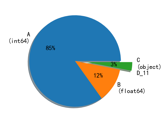
As shown in the above figure, D in 33 columns (the three columns with more missing values mentioned above will not be considered first)_ 11 is the object type. By looking at the data set, we find the variable D_ The data of 11 are as follows:

  

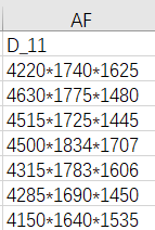
We can probably guess that variable D_11 represents the three dimensions of the car. So we deal with it and create three columns of length, width and height variables to split variable D_11. The code is as follows:

# Anonymous feature processing: D_11.  Split into length, width and high
series1 = Combine['D_11'].str.split('*', expand=True)
Combine['length'] = series1[0]
Combine['width'] = series1[1]
Combine['high'] = series1[2]

Combine['length'] = Combine['length'].astype(float)
Combine['width'] = Combine['width'].astype(float)
Combine['high'] = Combine['high'].astype(float)

Then we look at the data set. Among them, the variable carid represents the id number of the vehicle, which is a unique value, which is not helpful for our model training and can be deleted; Anonymous variable D_0, we use combine D_0.value_ Counts() to view the distribution of the variable value:

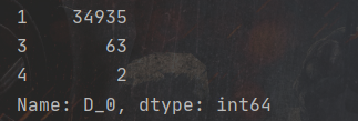
As can be seen from the above figure, variable D_0 has three values: 1, 3 and 4, but there are 34935 data with the value of one, accounting for more than 99%. Therefore, we can say: variable D_ The distribution of the value of 0 is extremely unbalanced and cannot provide useful information for model training. You can delete it.

After the above analysis, we will delete the variables to be deleted:

Combine.drop(['D_0', 'D_3', 'carid', 'D_6', 'D_11', 'D_14'], axis=1, inplace=True)  # Delete variables that are not conducive to model training

Where inplace=True indicates that the value of the original array is directly modified. The default is inplace=False, which means that you will get a return value after the drop operation. This return value is the modified array, that is, you need to define a new variable to receive the return value before you can get the modified array. If inplace=True, there is no need to receive the return value, and the target array will be modified directly.

2.3 characteristic Engineering

First, we use combine Nunique() check the number of different values of each variable:

        1. Discrete feature coding

According to the above figure, select the discrete variables' carcode ',' color ',' country ',' maketype ',' oiltype ',' D_ 7', 'D_ 8', 'D_ 9', 'D_ 10', 'D_ 13 'one hot encoding:

Define one hot encoding function:

def One_Hot(OneHotCol):
    new_cols = []
    for old_col in OneHotCol:
        new_cols += sorted(['{0}_{1}'.format(old_col, str(x).lower()) for x in set(Combine[old_col].values)])
    ec = OneHotEncoder()
    ec.fit(Combine[OneHotCol].values)
    # list(Combine.index.values)  # Take out the index of Combine
    OneHotCode = pd.DataFrame(ec.transform(Combine[OneHotCol]).toarray(), columns=new_cols,
                              index=list(Combine.index.values)).astype(int)
    return OneHotCode

Call the function written to encode the above discrete variables one hot:

OneHotCol = ['carCode', 'color', 'country', 'maketype', 'oiltype', 'D_7', 'D_8', 'D_9', 'D_10', 'D_13']
OneHotCode = One_Hot(OneHotCol)
# Merge Combine and OneHotCode
Combine = pd.concat([Combine, OneHotCode], axis=1)

Why use one hot coding? In short, it can be understood as: one hot coding expands the value of discrete features to the European space, and makes the distance between categories in discrete features equal in the European space, which is more reasonable than the ordinary coding method of categories with numbers. In this code, I use the OneHotEncoder() function in the preprocessing module of the sklearn library for one hot coding, so I need to guide the package.

        2. Date feature code

By looking at the dataset, we found the variables tradeTime, registerDtae, licenseDate, and D_12 all represent date information, so we can consider transforming them into the standard format of dates, and then extracting their year, month, day and week.

Date format conversion function (convert the date to the standard format of XXXX XX):

def date_proc(x):
    month = int(x[4:6])
    if month == 0:
        month = 1
    if len(x) == 6:
        return x[:4] + '-' + str(month)
    else:
        return x[:4] + '-' + str(month) + '-' + x[6:]

Date feature extraction function (extract the features of year, month, day and week):

def date_transform(df, fea_col):
    for f in tqdm(fea_col):
        df[f] = pd.to_datetime(df[f].astype('str').apply(date_proc))
        df[f + '_year'] = df[f].dt.year
        df[f + '_month'] = df[f].dt.month
        df[f + '_day'] = df[f].dt.day
        df[f + '_dayofweek'] = df[f].dt.dayofweek
    return (df)

The tqdm() function is used to add a progress bar, and the parameter is an iteratable object.

Perform standard date format conversion on the three variables' registerdate ',' tradetime 'and' licensedate 'and extract date features:

Date = ['registerDate', 'tradeTime', 'licenseDate']
Combine = date_transform(Combine, Date)

Due to variable D_ The date information represented by 12 is only year and month, so we extract the date feature separately after converting it to standard date format (only year and month are extracted):

# Anonymous feature processing D_ twelve
Combine = Combine[Combine['D_12'].notna()]
Combine['D_12'].astype('str').apply(date_proc)
Combine['D_12'] = pd.to_datetime(Train['D_12'])
Combine['D_12_year'] = Combine['D_12'].dt.year
Combine['D_12_month'] = Combine['D_12'].dt.month

After the above date features are extracted, the names of these feature variables in Combine are as follows:

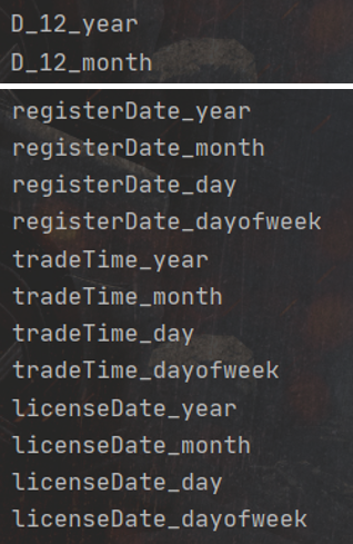
Similarly, call the one hot encoding function we wrote again to encode these features:

# The extracted date features are one hot coded
OneHotCol2 = ['registerDate_year', 'registerDate_month', 'registerDate_dayofweek', 'tradeTime_year', 'tradeTime_month',
             'tradeTime_dayofweek', 'licenseDate_year', 'licenseDate_month', 'licenseDate_dayofweek', 'D_12_year',
             'D_12_month']

OneHotCode2 = One_Hot(OneHotCol2)
Combine = pd.concat([Combine, OneHotCode2], axis=1)

        3. Build new features

Through the above date information variables, we can consider building some valuable new features. In this question, the characteristics I constructed are the number of days of use of the car, the number of days since the date of registration of the car, and the number of days since the date of launch of the car.

# Construction features: vehicle service days
Combine['used_time1'] = (pd.to_datetime(Combine['tradeTime'], format='%Y%m%d', errors='coerce') -
                      pd.to_datetime(Combine['registerDate'], format='%Y%m%d', errors='coerce')).dt.days
# Construction features: days from vehicle registration date
Combine['used_time2'] = (
        pd.datetime.now() - pd.to_datetime(Combine['registerDate'], format='%Y%m%d', errors='coerce')).dt.days
# Construction features: number of days from the date of vehicle launch
Combine['used_time3'] = (pd.datetime.now() - pd.to_datetime(Combine['tradeTime'], format='%Y%m%d', errors='coerce')).dt.days

        4. Bucket data

Write the date bucket function and_ time1', 'used_ time2', 'used_ Time3 'separate buckets:

# Data bucket function
def cut_group(df, cols, num_bins=50):
    for col in cols:
        all_range = int(df[col].max() - df[col].min())
        # ceil(): returns the uppermost integer of a number; floor(): returns the rounded down integer of a number
        bin = [np.ceil(df[col].min() - 1) + np.floor(i * all_range / num_bins) for i in range(num_bins + 2)]
        # Bin is a list, and the selection of both ends of the interval is determined according to the data in bin. For example, the first interval is [bin[0], bin[1]]
        df[col + '_bin'] = pd.cut(df[col], bin, labels=False)
    return df


# The data is divided into the number of days of use, the number of days from the date of registration and the number of days from the date of launch
CutCol = ['used_time1', 'used_time2', 'used_time3']
Combine = cut_group(Combine, CutCol, 50)

Data bucket division is a method of grouping multiple continuous values into a small number of "buckets", that is, the method of dividing multiple continuous values into intervals, which can reduce the amount of data.

        5. Feature Augmentation

Add anonymous features, multiply non anonymous features and anonymous features, and then obtain more information through feature expansion:

list1 = [1, 2, 4, 5, 7, 8, 9, 10, 12, 13]
for i in ['D_' + str(m) for m in list1]:
    for j in ['D_' + str(n) for n in list1]:
        Combine[str(i) + '+' + str(j)] = Combine[i] + Combine[j]
for i in ['brand', 'serial', 'model', 'mileage', 'color', 'cityId', 'carCode', 'transferCount', 'seatings', 'country',
          'maketype', 'modelyear', 'displacement', 'gearbox', 'oiltype', 'newprice', 'length', 'width', 'high']:
    for j in ['D_' + str(n) for n in list1]:
        Combine[str(i) + '*' + str(j)] = Combine[i] * Combine[j]

        6. Feature crossover

First, let's analyze the correlation between anonymous variables and non anonymous variables and price:

AllCol = Combine.columns
Train = Combine.iloc[:len(Train), :][AllCol]
a = dict(Train.corr()['price'])  # Correlation between each variable and price variable
asortlist = sorted(a.items(), key=lambda x: x[1], reverse=True)  # Sort the items of the dictionary based on the value of the dictionary
for i in asortlist:
    print(i)

I rank the variables from high to low according to their correlation with the price variable, as shown in the following figure:

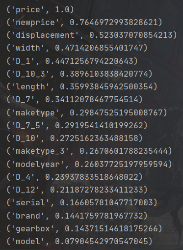
In the figure above, the larger the value after the variable name, the greater the correlation with price. Then, we select anonymous variables and non anonymous variables that have a large correlation with price, and let them cross the features to obtain more complex nonlinear features:

# Characteristic cross function
def cross_feature(df, fea_col, Nfea_col):
    for i in tqdm(fea_col):  # Ergodic classification feature
        for j in tqdm(Nfea_col):  # Ergodic numerical characteristics
            # Call the groupby() function to group the data with parameter i, and then use the agg function to aggregate the data (find the maximum, minimum and median)
            feat = df.groupby(i, as_index=False)[j].agg({
                '{}_{}_max'.format(i, j): 'max',  # Maximum
                '{}_{}_min'.format(i, j): 'min',  # minimum value
                '{}_{}_median'.format(i, j): 'median',  # median
            })
            df = df.merge(feat, on=i, how='left')
    return (df)


# Non anonymous variables and anonymous variables with high correlation with Price are selected for feature crossover
Cross_fea = ['newprice', 'displacement', 'width', 'length', 'maketype', 'maketype_3', 'modelyear']
Cross_Nfea = ['D_1', 'D_10_3', 'D_7', 'D_7_5', 'D_10', 'D_4', 'D_12']
Combine = cross_feature(Combine, Cross_fea, Cross_Nfea)

After the above operations, in order to facilitate the following operations, restore the training set and test set first:

# Restore training and test sets
InputCol = Combine.columns.drop('price')
XTrain = Combine.iloc[:len(Train), :][InputCol]
YTrain = Train['price']
XTest = Combine.iloc[len(Train):, :][InputCol]

print("XTrain shape: ", XTrain.shape)
print("XTestshape: ", XTest.shape)

        7. Average coding

For high cardinality features, average coding can be used to supervise and determine the coding method most suitable for this qualitative feature. High cardinality feature is simply a feature with many values. For these features that are not suitable for one hot coding, the concept of average coding was proposed. If you want to know more about the average code, you can take a look at this blog. I just copy the average code written by this big man:

Average coding: data preprocessing / Feature Engineering for high cardinality qualitative features (category features) https://blog.csdn.net/juzexia/article/details/78581462?spm=1001.2014.3001.5506 Average coding implementation code:

class MeanEncoder:
    def __init__(self, categorical_features, n_splits=10, target_type='classification', prior_weight_func=None):
        self.categorical_features = categorical_features
        self.n_splits = n_splits
        self.learned_stats = {}

        if target_type == 'classification':
            self.target_type = target_type
            self.target_values = []
        else:
            self.target_type = 'regression'
            self.target_values = None

        if isinstance(prior_weight_func, dict):
            self.prior_weight_func = eval('lambda x: 1 / (1 + np.exp((x - k) / f))', dict(prior_weight_func, np=np))
        elif callable(prior_weight_func):
            self.prior_weight_func = prior_weight_func
        else:
            self.prior_weight_func = lambda x: 1 / (1 + np.exp((x - 2) / 1))

    @staticmethod
    def mean_encode_subroutine(X_train, y_train, X_test, variable, target, prior_weight_func):

        X_train = X_train[[variable]].copy()
        X_test = X_test[[variable]].copy()

        if target is not None:
            nf_name = '{}_pred_{}'.format(variable, target)
            X_train['pred_temp'] = (y_train == target).astype(int)  # classification
        else:
            nf_name = '{}_pred'.format(variable)
            X_train['pred_temp'] = y_train  # regression
        prior = X_train['pred_temp'].mean()

        col_avg_y = X_train.groupby(variable)['pred_temp'].agg(['mean', 'size']).rename(
            columns={'mean': 'mean', 'size': 'beta'})
        col_avg_y['beta'] = prior_weight_func(col_avg_y['beta'])
        col_avg_y[nf_name] = col_avg_y['beta'] * prior + (1 - col_avg_y['beta']) * col_avg_y['mean']
        col_avg_y.drop(['beta', 'mean'], axis=1, inplace=True)

        nf_train = X_train.join(col_avg_y, on=variable)[nf_name].values
        nf_test = X_test.join(col_avg_y, on=variable).fillna(prior, inplace=False)[nf_name].values

        return nf_train, nf_test, prior, col_avg_y

    def fit_transform(self, X, y):
        X_new = X.copy()
        if self.target_type == 'classification':
            skf = StratifiedKFold(self.n_splits)
        else:
            skf = KFold(self.n_splits)

        if self.target_type == 'classification':
            self.target_values = sorted(set(y))
            self.learned_stats = {'{}_pred_{}'.format(variable, target): [] for variable, target in
                                  product(self.categorical_features, self.target_values)}
            for variable, target in product(self.categorical_features, self.target_values):
                nf_name = '{}_pred_{}'.format(variable, target)
                X_new.loc[:, nf_name] = np.nan
                for large_ind, small_ind in skf.split(y, y):
                    nf_large, nf_small, prior, col_avg_y = MeanEncoder.mean_encode_subroutine(
                        X_new.iloc[large_ind], y.iloc[large_ind], X_new.iloc[small_ind], variable, target,
                        self.prior_weight_func)
                    X_new.iloc[small_ind, -1] = nf_small
                    self.learned_stats[nf_name].append((prior, col_avg_y))
        else:
            self.learned_stats = {'{}_pred'.format(variable): [] for variable in self.categorical_features}
            for variable in self.categorical_features:
                nf_name = '{}_pred'.format(variable)
                X_new.loc[:, nf_name] = np.nan
                for large_ind, small_ind in skf.split(y, y):
                    nf_large, nf_small, prior, col_avg_y = MeanEncoder.mean_encode_subroutine(
                        X_new.iloc[large_ind], y.iloc[large_ind], X_new.iloc[small_ind], variable, None,
                        self.prior_weight_func)
                    X_new.iloc[small_ind, -1] = nf_small
                    self.learned_stats[nf_name].append((prior, col_avg_y))
        return X_new

    def transform(self, X):
        X_new = X.copy()

        if self.target_type == 'classification':
            for variable, target in product(self.categorical_features, self.target_values):
                nf_name = '{}_pred_{}'.format(variable, target)
                X_new[nf_name] = 0
                for prior, col_avg_y in self.learned_stats[nf_name]:
                    X_new[nf_name] += X_new[[variable]].join(col_avg_y, on=variable).fillna(prior, inplace=False)[
                        nf_name]
                X_new[nf_name] /= self.n_splits
        else:
            for variable in self.categorical_features:
                nf_name = '{}_pred'.format(variable)
                X_new[nf_name] = 0
                for prior, col_avg_y in self.learned_stats[nf_name]:
                    X_new[nf_name] += X_new[[variable]].join(col_avg_y, on=variable).fillna(prior, inplace=False)[
                        nf_name]
                X_new[nf_name] /= self.n_splits

        return X_new

Then, average coding is performed for some features:

MeanEncol = ['model', 'brand', 'registerDate', 'tradeTime']
# If it is a regression scenario, target_type='regression'; If it is a classified scene, target_type='classification'
MeanFit = MeanEncoder(MeanEncol, target_type='regression')
XTrain = MeanFit.fit_transform(XTrain, YTrain)
XTest = MeanFit.transform(XTest)

        8. Target coding

Target code is a kind of code based on the corresponding relationship between features and target values. The figure below shows the K-fold target code. The K-fold target code divides the samples to be coded into K parts. The target code of each sample uses the corresponding attributes of those samples of the same category in the other K-1 data, such as maximum and minimum values, Better than ordinary target coding.

# K-fold target code,
# In regression scenarios, common methods of target coding: minimum, maximum, median, mean, sum, standard deviation, skewness, kurtosis and median absolute deviation
XTrain['price'] = Train['price']
EncCol = []
StatDefaultDict = {
    'max': XTrain['price'].max(),
    'min': XTrain['price'].min(),
    'median': XTrain['price'].median(),
    'mean': XTrain['price'].mean(),
    'sum': XTrain['price'].sum(),
    'std': XTrain['price'].std(),
    'skew': XTrain['price'].skew(),
    'kurt': XTrain['price'].kurt(),
    'mad': XTrain['price'].mad()
}
# The maximum value, minimum value and mean value are used to encode the target feature price respectively

EncStat = ['max', 'min', 'mean']
# 10% off
KF = KFold(n_splits=10, shuffle=True, random_state=2022)
for f in tqdm(['serial', 'brand', 'registerDate_year', 'tradeTime_year', 'mileage', 'model']):
    EncDict = {}
    for stat in EncStat:
        EncDict['{}_target_{}'.format(f, stat)] = stat
        XTrain['{}_target_{}'.format(f, stat)] = 0
        XTest['{}_target_{}'.format(f, stat)] = 0
        EncCol.append('{}_target_{}'.format(f, stat))
    for i, (TrnIndex, ValIndex) in enumerate(KF.split(XTrain, YTrain)):
        TrnX, ValX = XTrain.iloc[TrnIndex].reset_index(drop=True), XTrain.iloc[ValIndex].reset_index(drop=True)
        EncDF = TrnX.groupby(f, as_index=False)['price'].agg(EncDict)
        ValX = ValX[[f]].merge(EncDF, on=f, how='left')
        TestX = XTest[[f]].merge(EncDF, on=f, how='left')
        for stat in EncStat:
            ValX['{}_target_{}'.format(f, stat)] = ValX['{}_target_{}'.format(f, stat)].fillna(StatDefaultDict[stat])
            TestX['{}_target_{}'.format(f, stat)] = TestX['{}_target_{}'.format(f, stat)].fillna(StatDefaultDict[stat])
            XTrain.loc[ValIndex, '{}_target_{}'.format(f, stat)] = ValX['{}_target_{}'.format(f, stat)].values
            XTest['{}_target_{}'.format(f, stat)] += TestX['{}_target_{}'.format(f, stat)].values / KF.n_splits

After the above process, let's check the dimensions of the current data:

print("XTrain shape: ", XTrain.shape)
print("XTest shape: ", XTest.shape)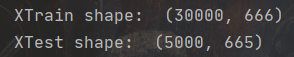

3, Dimensionality reduction

As can be seen from the above figure, the number of features has reached 666 now, but if all these are fed to the model, some useless features may affect our model training, so we need to reduce the dimension, retain the main feature scores to the greatest extent and screen out the noise.

In this code, I use PCA dimensionality reduction. As for the dimensionality reduction steps of PCA, I said in my last article, so this time I will be simpler.

Firstly, in order to ensure that the scale of feature measurement is consistent, we use range method to normalize features.

The normalization formula is as follows:

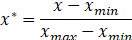
In the above formula,Is the maximum value of sample data,Is the minimum value of sample data.

Based on the above analysis, we first call the MinMaxScalar() function in the preprocessing module in the sklearn library to normalize the features, and then call the PCA algorithm package in the decomposition module in the sklearn library to reduce the dimension of the data. The steps are:

1. De averaging:

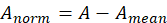
Among them,Is the standardized matrix, Is the mean of matrix A.

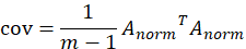
2. Find the covariance matrix of the standardized data set:

3. Calculate the eigenvalues and eigenvectors of the covariance matrix. Set number λ And n-dimensional non-0 column vector x satisfy the following formula:

Then λ Is the eigenvalue of C, and x is the corresponding eigenvalue of C λ Eigenvector of. C is the covariance matrix of the data set.

4. Retain the first k most important features. K is the dimension you want to reduce to.

5. Find the eigenvector corresponding to these k eigenvalues

6. Multiply the standardized data set by these k eigenvectors to obtain the dimension reduction result

In the above formula,Represents a matrix composed of eigenvectors corresponding to the above k eigenvalues.

The implementation of the above complete process code is as follows:

# Normalization (range method)
Scaler = MinMaxScaler()
Scaler.fit(pd.concat([XTrain, XTest]).values)
CombineScaler = Scaler.transform(pd.concat([XTrain, XTest]).values)
print('CombineScaler shape: ', CombineScaler.shape)
# Call the PCA algorithm package in the decomposition module in the sklearn library to reduce the dimension of the data
# PCA dimensionality reduction
PCA = decomposition.PCA(n_components=550)
CombinePCA = PCA.fit_transform(CombineScaler)
XTrainPCA = CombinePCA[:len(XTrain)]
XTestPCA = CombinePCA[len(XTrain):]

YTrain = Train['price'].values
print('CombinePCA shape: ', CombinePCA.shape)

IV. model establishment

This neural network model, I use a neural network defined by the boss, and the use effect is OK.

def NN_model(input_dim):
    # Parameter random initialization
    init = keras.initializers.glorot_uniform(seed=1)
    model = keras.models.Sequential()
    model.add(Dense(units=300, use_bias=True, input_dim=input_dim, kernel_initializer=init, activation='softplus'))
    model.add(Dense(units=300, use_bias=True, kernel_initializer=init, activation='softplus'))  # ReLU
    model.add(Dense(units=64, use_bias=True, kernel_initializer=init, activation='softplus'))
    model.add(Dense(units=32, use_bias=True, kernel_initializer=init, activation='softplus'))
    model.add(Dense(units=8, use_bias=True, kernel_initializer=init, activation='softplus'))
    model.add(Dense(units=1))
    return model


class Metric(Callback):
    def __init__(self, model, callbacks, Combine):
        super().__init__()
        self.model = model
        self.callbacks = callbacks
        self.Combine = Combine

    def on_train_begin(self, logs=None):
        for callback in self.callbacks:
            callback.on_train_begin(logs)

    def on_train_end(self, logs=None):
        for callback in self.callbacks:
            callback.on_train_end(logs)

    def on_epoch_end(self, batch, logs=None):
        X_train, y_train = self.Combine[0][0], self.Combine[0][1]
        y_pred3 = self.model.predict(X_train)
        y_pred = np.zeros((len(y_pred3),))
        y_true = np.zeros((len(y_pred3),))
        for i in range(len(y_pred3)):
            y_pred[i] = y_pred3[i]
        for i in range(len(y_pred3)):
            y_true[i] = y_train[i]
        trn_s = metrics.mean_absolute_error(y_true, y_pred)
        logs['trn_score'] = trn_s

        X_val, y_val = self.Combine[1][0], self.Combine[1][1]
        y_pred3 = self.model.predict(X_val)
        y_pred = np.zeros((len(y_pred3),))
        y_true = np.zeros((len(y_pred3),))
        for i in range(len(y_pred3)):
            y_pred[i] = y_pred3[i]
        for i in range(len(y_pred3)):
            y_true[i] = y_val[i]
        val_s = metrics.mean_absolute_error(y_true, y_pred)

        logs['val_score'] = val_s
        print('trn_score', trn_s, 'val_score', val_s)

        for callback in self.callbacks:
            callback.on_epoch_end(batch, logs)

I drew the structure diagram of the neural network model, which is roughly as follows:

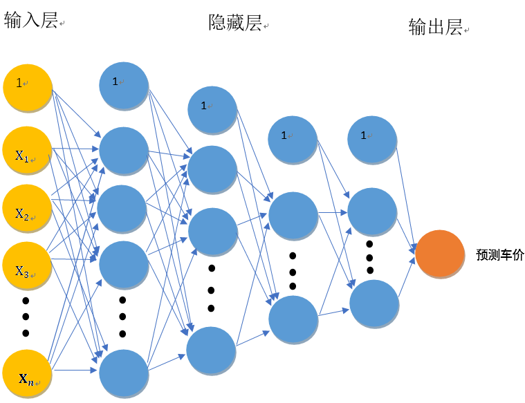
Because there are many neurons, the weight w is not marked in the figure. Let me briefly introduce this neural network with my own understanding:

In this neural network, artificial neurons can accept n real value inputs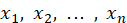, they form the input vector. The next level of input is a linear unit. The output of the linear unit is:

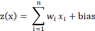
         It is the offset term, which can be understood as the intercept on the y-axis. If there is no offset term, the neuron will never fit the function that is not the origin.Enter the corresponding weight for the ith. For the convenience of expression, we make=bias, and add a feature with a value of 1 to the input vector, the output is:

                                                              

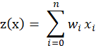
It can be seen thatIt is a simulation of the potential level of neurons, andIs the threshold. The single value output of the linear unit will be sent to the next level activation unit (activation function). The activation function we choose is softplus function, and the mathematical expression of this function is:

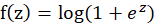
Therefore, the final output function of neurons is:

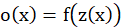
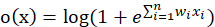
Substitute in:

The loss function we choose is MAE (mean absolute error), and its error is calculated as follows:

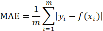
Where, m represents the number of sample points,Represents the i th true value,The ith represents the predicted value. In neural network, the loss function is to calculate the error, and then update the weight in neural network training according to the error.

5, Model training

Dynamically adjust learning rate:

def scheduler(epoch):
    # Every 20 epoch s, the learning rate is reduced to half of the original
    if epoch % 20 == 0 and epoch != 0:
        lr = K.get_value(model.optimizer.lr)
        K.set_value(model.optimizer.lr, lr * 0.5)
        print("lr changed to {}".format(lr * 0.5))
    return K.get_value(model.optimizer.lr)


reduce_lr = LearningRateScheduler(scheduler)

Model training:

N = 10  # 10% off cross validation
kfold = KFold(n_splits=N, shuffle=True)
BSize = 2000
MaxEpochs = 140
RinPred = np.zeros((len(XTrainPCA),))

for fold, (trn_idx, val_idx) in enumerate(kfold.split(XTrainPCA, YTrain)):
    print('fold:', fold+1)
    X_train, y_train = XTrainPCA[trn_idx], YTrain[trn_idx]
    X_val, y_val = XTrainPCA[val_idx], YTrain[val_idx]

    model = NN_model(X_train.shape[1])
    # The learning rate is initially set to 0.01
    simple_adam = Adam(lr=0.01)
    model.compile(loss='mae', optimizer=simple_adam, metrics=['mae'])
    es = EarlyStopping(monitor='val_score', patience=10, verbose=1, mode='min', restore_best_weights=True, )
    es.set_model(model)
    metric = Metric(model, [es], [(X_train, y_train), (X_val, y_val)])
    # batch_size: batch is required for each weight update_ Size data is calculated to obtain the loss function, and each operation batch_size data is equivalent to one iteration. Each iteration will update the weight of the parameter.
    # Epochs: defined as a single training iteration of all batches in forward and backward propagation. In short, epochs refers to how many times the data will be "rotated" during the training process
    # Assuming that the training set has 1000 samples and batchsize=10, training a complete sample set requires 100 iteration s and 1 epoch
    model.fit(X_train, y_train, batch_size=BSize, epochs=MaxEpochs,
              validation_data=(X_val, y_val),
              callbacks=[reduce_lr], shuffle=True, verbose=1)
    y_pred3 = model.predict(X_val)
    y_pred = np.zeros((len(y_pred3),))
    for i in range(len(y_pred3)):
        y_pred[i] = y_pred3[i]
    RinPred[val_idx] = y_pred

    np.set_printoptions(suppress=True)  # Not output by scientific counting method
    # True value of training set
    # print(np.around(YTrain[val_idx], 2))
    # Training set prediction
    # print(np.around(y_pred, 2))
    # Output the predicted value of used car price in data2
    print(np.around(model.predict(XTestPCA), 2))
    print(Evaluate(YTrain[val_idx], y_pred))

In model training, we use Adam as the optimizer. According to the loss function, the neural network will use Adam optimizer and back-propagation algorithm to update the weight of network parameters, so as to train the network model and optimize the neural network. The formula of weight updating by Adam optimizer is complex, so I won't list it. If you want to know, you can find it by searching on the Internet.

According to the model evaluation criteria given by the title:

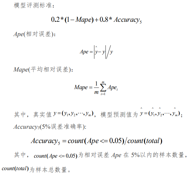
Define model evaluation function:

#  evaluation model 
def Evaluate(y_tre, y_pre):
# y_tre: true value; y_pre: predicted value
    m = len(y_tre)
    count1 = 0
    Ape = []
    for i in range(0, m):
        Ape.append(np.abs(y_pre[i] - y_tre[i]) / y_tre[i])
    Mape = sum(Ape) / m

    for i in Ape:
        if i <= 0.05:
            count1 += 1

    Accuracy = count1 / m
    print('Mape:', Mape)
    print('Accuracy', Accuracy)
    print('score', 0.2 * (1 - Mape) + 0.8 * Accuracy)

Run the code. According to the evaluation function, the better result is:

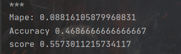
In order to better display the prediction results of the model, I randomly selected some data in the training set and compared their real values with the predicted values. After visualization, it is shown in the following figure:

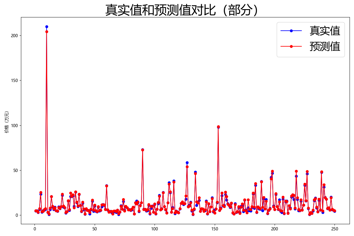
It can be seen that the overall prediction result of the model is good.

I put the complete code in the following link, 0 points, if necessary, you can download it yourself.

python implementation of price prediction using neural network in machine learning - machine learning document resources - CSDN Library https://download.csdn.net/download/qq_48958559/77393492https://download.csdn.net/download/qq_48958559/77393492 I have just begun to contact machine learning. If there are mistakes, I hope I can correct them.