Python mathematical modeling series: differential equations

preface

Hello! buddy!
Thank you very much for reading Haihong's article. If there are mistakes in the article, you are welcome to point out ~

Self introduction ˊ ᵕ ˋ) ੭
Nickname: Hai Hong
Label: program ape ｜ C + + player ｜ student
Introduction: I got acquainted with programming in C language and then transferred to computer major. I was lucky to have won some national and provincial awards... And I have been guaranteed to study. Currently learning C++/Linux/Python
Learning experience: solid foundation + taking more notes + typing more codes + thinking more + learning English well!

Beginner Python Xiaobai stage
The article is only used as your own learning notes for knowledge system establishment and review
The problem is not to learn one more problem and understand one more problem
Know it, know why!

Python mathematical modeling series (1): linear programming of programming problems

Python mathematical modeling series (2): integer programming of programming problems

Python mathematical modeling series (3): nonlinear programming of planning problems

Python mathematical modeling series (4): numerical approximation

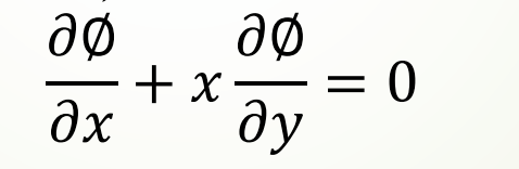
1. Classification of differential equations

Differential equation is an equation used to describe the relationship between a certain kind of function and its derivative, and its solution is a function conforming to the equation.

Differential equations can be divided into ordinary differential equations and partial differential equations according to the number of independent variables

ordinary differential equation (ODE)

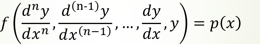
Partial differential equation (more than two independent variables)

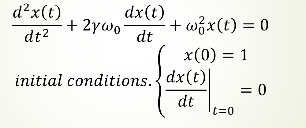
2. Analytical solutions of differential equations

ODE (ordinary differential equation) with analytical solution can be solved by using SymPy library

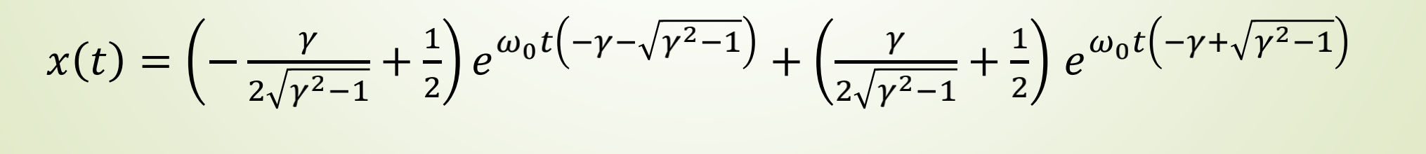
Taking the second-order ODE of a damped harmonic oscillator as an example, the expression is:

Demo code

import sympy
 
 
def apply_ics(sol, ics, x, known_params):
    free_params = sol.free_symbols - set(known_params)
    eqs = [(sol.lhs.diff(x, n) - sol.rhs.diff(x, n)).subs(x, 0).subs(ics) for n in range(len(ics))]
    sol_params = sympy.solve(eqs, free_params)
    return sol.subs(sol_params)
 
 
# Initialize print environment
sympy.init_printing()
# Mark the parameters and they are all positive
t, omega0, gamma = sympy.symbols("t, omega_0, gamma", positive=True)
# Mark x is a differential function, not a variable
x = sympy.Function("x")
# The general solution is obtained by diff() and dsolve 
# ode differential equation is the part to the left of the equal sign and 0 to the right of the equal sign
ode = x(t).diff(t, 2) + 2 * gamma * omega0 * x(t).diff(t) + omega0 ** 2 * x(t)
ode_sol = sympy.dsolve(ode)
# Initial condition: dictionary matching
ics = {x(0): 1, x(t).diff(t).subs(t, 0): 0}
x_t_sol = apply_ics(ode_sol, ics, t, [omega0, gamma])
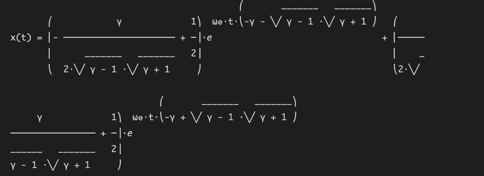
sympy.pprint(x_t_sol)

Operation results:

3. Numerical solution of differential equation

When ODE cannot obtain an analytical solution, you can use integrate. In scipy Odeint seeks the numerical solution to explore some properties of its solution, supplemented by visualization, which can intuitively show the functional expression of ODE solution.

Take the following first-order nonlinear (because the power of function y is 2) ODE as an example:

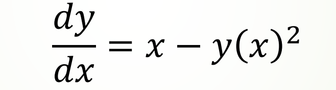
Now we use odeint to find its numerical solution

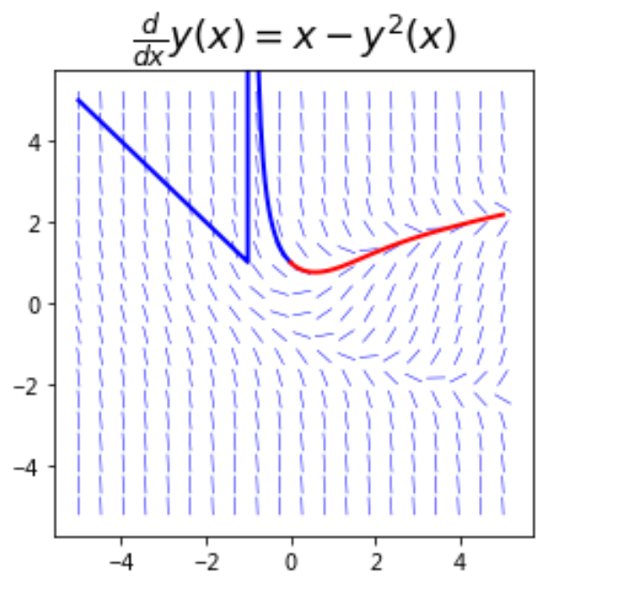
3.1 field line diagram and numerical solution

Demo code

import numpy as np
from scipy import integrate
import matplotlib.pyplot as plt
import sympy

def plot_direction_field(x, y_x, f_xy, x_lim=(-5, 5), y_lim=(-5, 5), ax=None):
    f_np = sympy.lambdify((x, y_x), f_xy, 'numpy')
    x_vec = np.linspace(x_lim[0], x_lim[1], 20)
    y_vec = np.linspace(y_lim[0], y_lim[1], 20)

    if ax is None:
        _, ax = plt.subplots(figsize=(4, 4))

    dx = x_vec[1] - x_vec[0]
    dy = y_vec[1] - y_vec[0]

    for m, xx in enumerate(x_vec):
        for n, yy in enumerate(y_vec):
            Dy = f_np(xx, yy) * dx
            Dx = 0.8 * dx**2 / np.sqrt(dx**2 + Dy**2)
            Dy = 0.8 * Dy*dy / np.sqrt(dx**2 + Dy**2)
            ax.plot([xx - Dx/2, xx + Dx/2], [yy - Dy/2, yy + Dy/2], 'b', lw=0.5)

    ax.axis('tight')
    ax.set_title(r"$%s$" %(sympy.latex(sympy.Eq(y_x.diff(x), f_xy))), fontsize=18)

    return ax

x = sympy.symbols('x')
y = sympy.Function('y')
f = x-y(x)**2

f_np = sympy.lambdify((y(x), x), f)
## put variables (y(x), x) into lambda function f.
y0 = 1
xp = np.linspace(0, 5, 100)
yp = integrate.odeint(f_np, y0, xp)
## solve f_np with initial conditons y0, and x ranges as xp.
xn = np.linspace(0, -5, 100)
yn = integrate.odeint(f_np, y0, xn)

fig, ax = plt.subplots(1, 1, figsize=(4, 4))
plot_direction_field(x, y(x), f, ax=ax)
## plot direction field of function f
ax.plot(xn, yn, 'b', lw=2)
ax.plot(xp, yp, 'r', lw=2)
plt.show()

Operation results:

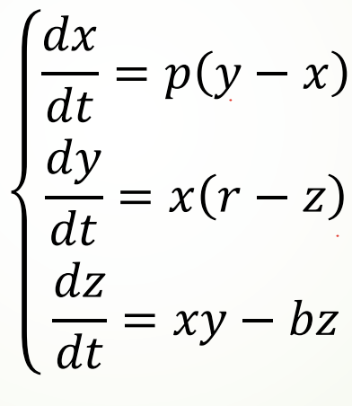
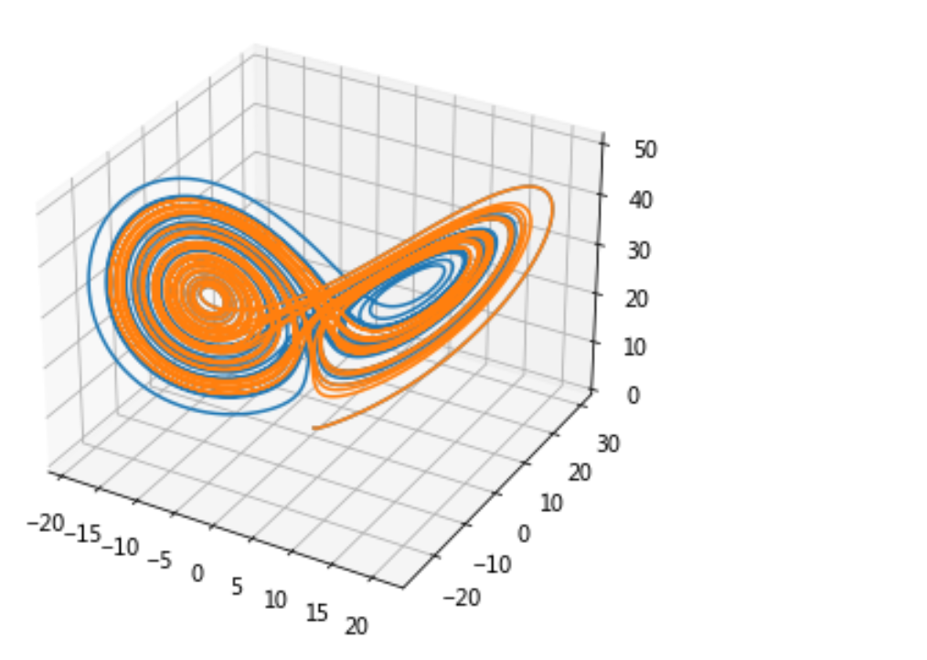
3.2 Lorentz curve and numerical solution

Taking solving the Lorentz curve as an example, the following equations represent the speed of the curve in xyz three directions. Given an initial point, the corresponding Lorentz curve can be drawn:

Demo code

import numpy as np
from scipy.integrate import odeint
from mpl_toolkits.mplot3d import Axes3D
import matplotlib.pyplot as plt
 
 
def dmove(Point, t, sets):
    p, r, b = sets
    x, y, z = Point
    return np.array([p * (y - x), x * (r - z), x * y - b * z])
 
 
t = np.arange(0, 30, 0.001)
P1 = odeint(dmove, (0., 1., 0.), t, args=([10., 28., 3.],))
P2 = odeint(dmove, (0., 1.01, 0.), t, args=([10., 28., 3.],))
fig = plt.figure()
ax = Axes3D(fig)
ax.plot(P1[:, 0], P1[:, 1], P1[:, 2])
ax.plot(P2[:, 0], P2[:, 1], P2[:, 2])
plt.show()

Operation results:

4. Infectious disease model

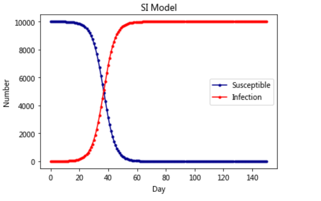
Model 1: Si model

import scipy.integrate as spi
import numpy as np
import matplotlib.pyplot as plt

# N is the total number of people
N = 10000
# β Is the infection rate coefficient
beta = 0.25
# gamma is the recovery coefficient
gamma = 0
# I_0 is the initial number of infected persons
I_0 = 1
# S_0 is the initial number of susceptible people
S_0 = N - I_0
# T is the propagation time
T = 150

# INI is the array in the initial state
INI = (S_0,I_0)


def funcSI(inivalue,_):
    Y = np.zeros(2)
    X = inivalue
    # Susceptible individual change
    Y[0] = - (beta * X[0] * X[1]) / N + gamma * X[1]
    # Individual change of infection
    Y[1] = (beta * X[0] * X[1]) / N - gamma * X[1]
    return Y

T_range = np.arange(0,T + 1)

RES = spi.odeint(funcSI,INI,T_range)


plt.plot(RES[:,0],color = 'darkblue',label = 'Susceptible',marker = '.')
plt.plot(RES[:,1],color = 'red',label = 'Infection',marker = '.')
plt.title('SI Model')
plt.legend()
plt.xlabel('Day')
plt.ylabel('Number')
plt.show()

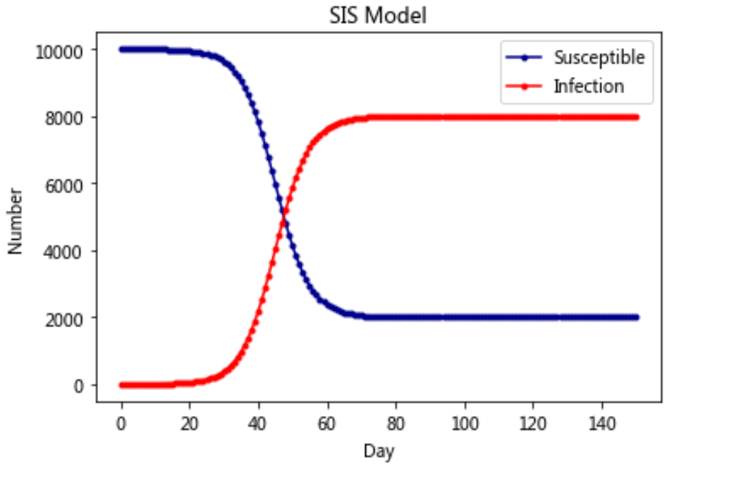
Model 2: SIS model

import scipy.integrate as spi
import numpy as np
import matplotlib.pyplot as plt

# N is the total number of people
N = 10000
# β Is the infection rate coefficient
beta = 0.25
# gamma is the recovery coefficient
gamma = 0.05
# I_0 is the initial number of infected persons
I_0 = 1
# S_0 is the initial number of susceptible people
S_0 = N - I_0
# T is the propagation time
T = 150

# INI is the array in the initial state
INI = (S_0,I_0)


def funcSIS(inivalue,_):
    Y = np.zeros(2)
    X = inivalue
    # Susceptible individual change
    Y[0] = - (beta * X[0]) / N * X[1] + gamma * X[1]
    # Individual change of infection
    Y[1] = (beta * X[0] * X[1]) / N - gamma * X[1]
    return Y

T_range = np.arange(0,T + 1)

RES = spi.odeint(funcSIS,INI,T_range)

plt.plot(RES[:,0],color = 'darkblue',label = 'Susceptible',marker = '.')
plt.plot(RES[:,1],color = 'red',label = 'Infection',marker = '.')
plt.title('SIS Model')
plt.legend()
plt.xlabel('Day')
plt.ylabel('Number')
plt.show()

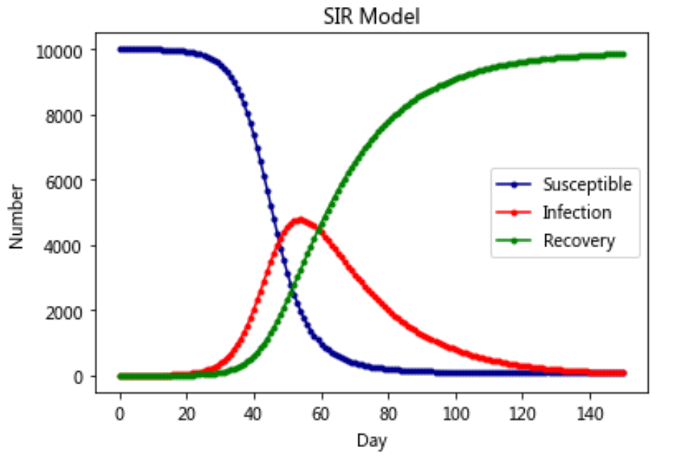
Model 3: SIR model

import scipy.integrate as spi
import numpy as np
import matplotlib.pyplot as plt

# N is the total number of people
N = 10000
# β Is the infection rate coefficient
beta = 0.25
# gamma is the recovery coefficient
gamma = 0.05
# I_0 is the initial number of infected persons
I_0 = 1
# R_0 is the initial number of healers
R_0 = 0
# S_0 is the initial number of susceptible people
S_0 = N - I_0 - R_0
# T is the propagation time
T = 150

# INI is the array in the initial state
INI = (S_0,I_0,R_0)


def funcSIR(inivalue,_):
    Y = np.zeros(3)
    X = inivalue
    # Susceptible individual change
    Y[0] = - (beta * X[0] * X[1]) / N
    # Individual change of infection
    Y[1] = (beta * X[0] * X[1]) / N - gamma * X[1]
    # Cure individual changes
    Y[2] = gamma * X[1]
    return Y

T_range = np.arange(0,T + 1)

RES = spi.odeint(funcSIR,INI,T_range)


plt.plot(RES[:,0],color = 'darkblue',label = 'Susceptible',marker = '.')
plt.plot(RES[:,1],color = 'red',label = 'Infection',marker = '.')
plt.plot(RES[:,2],color = 'green',label = 'Recovery',marker = '.')
plt.title('SIR Model')
plt.legend()
plt.xlabel('Day')
plt.ylabel('Number')
plt.show()

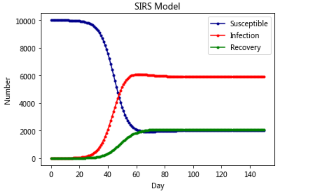
Model 4: SIRS model

import scipy.integrate as spi
import numpy as np
import matplotlib.pyplot as plt

# N is the total number of people
N = 10000
# β Is the infection rate coefficient
beta = 0.25
# gamma is the recovery coefficient
gamma = 0.05
# Ts is the antibody duration
Ts = 7
# I_0 is the initial number of infected persons
I_0 = 1
# R_0 is the initial number of healers
R_0 = 0
# S_0 is the initial number of susceptible people
S_0 = N - I_0 - R_0
# T is the propagation time
T = 150

# INI is the array in the initial state
INI = (S_0,I_0,R_0)


def funcSIRS(inivalue,_):
    Y = np.zeros(3)
    X = inivalue
    # Susceptible individual change
    Y[0] = - (beta * X[0] * X[1]) / N + X[2] / Ts
    # Individual change of infection
    Y[1] = (beta * X[0] * X[1]) / N - gamma * X[1]
    # Cure individual changes
    Y[2] = gamma * X[1] - X[2] / Ts
    return Y

T_range = np.arange(0,T + 1)

RES = spi.odeint(funcSIRS,INI,T_range)


plt.plot(RES[:,0],color = 'darkblue',label = 'Susceptible',marker = '.')
plt.plot(RES[:,1],color = 'red',label = 'Infection',marker = '.')
plt.plot(RES[:,2],color = 'green',label = 'Recovery',marker = '.')
plt.title('SIRS Model')
plt.legend()
plt.xlabel('Day')
plt.ylabel('Number')
plt.show()

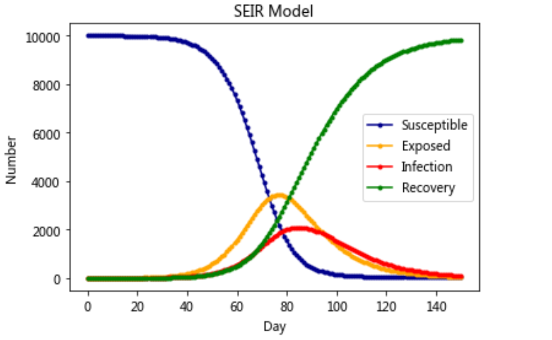
Model 5: SEIR model

import scipy.integrate as spi
import numpy as np
import matplotlib.pyplot as plt

# N is the total number of people
N = 10000
# β Is the infection rate coefficient
beta = 0.6
# gamma is the recovery coefficient
gamma = 0.1
# Te is the disease incubation period
Te = 14
# I_0 is the initial number of infected persons
I_0 = 1
# E_0 is the initial number of lurks
E_0 = 0
# R_0 is the initial number of healers
R_0 = 0
# S_0 is the initial number of susceptible people
S_0 = N - I_0 - E_0 - R_0
# T is the propagation time
T = 150

# INI is the array in the initial state
INI = (S_0,E_0,I_0,R_0)


def funcSEIR(inivalue,_):
    Y = np.zeros(4)
    X = inivalue
    # Susceptible individual change
    Y[0] = - (beta * X[0] * X[2]) / N
    # Latent individual change
    Y[1] = (beta * X[0] * X[2]) / N - X[1] / Te
    # Individual change of infection
    Y[2] = X[1] / Te - gamma * X[2]
    # Cure individual changes
    Y[3] = gamma * X[2]
    return Y

T_range = np.arange(0,T + 1)

RES = spi.odeint(funcSEIR,INI,T_range)


plt.plot(RES[:,0],color = 'darkblue',label = 'Susceptible',marker = '.')
plt.plot(RES[:,1],color = 'orange',label = 'Exposed',marker = '.')
plt.plot(RES[:,2],color = 'red',label = 'Infection',marker = '.')
plt.plot(RES[:,3],color = 'green',label = 'Recovery',marker = '.')

plt.title('SEIR Model')
plt.legend()
plt.xlabel('Day')
plt.ylabel('Number')
plt.show()

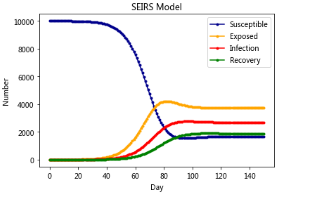
Model 6: SEIRS model

import scipy.integrate as spi
import numpy as np
import matplotlib.pyplot as plt

# N is the total number of people
N = 10000
# β Is the infection rate coefficient
beta = 0.6
# gamma is the recovery coefficient
gamma = 0.1
# Ts is the antibody duration
Ts = 7
# Te is the disease incubation period
Te = 14
# I_0 is the initial number of infected persons
I_0 = 1
# E_0 is the initial number of lurks
E_0 = 0
# R_0 is the initial number of healers
R_0 = 0
# S_0 is the initial number of susceptible people
S_0 = N - I_0 - E_0 - R_0
# T is the propagation time
T = 150

# INI is the array in the initial state
INI = (S_0,E_0,I_0,R_0)


def funcSEIRS(inivalue,_):
    Y = np.zeros(4)
    X = inivalue
    # Susceptible individual change
    Y[0] = - (beta * X[0] * X[2]) / N + X[3] / Ts
    # Latent individual change
    Y[1] = (beta * X[0] * X[2]) / N - X[1] / Te
    # Individual change of infection
    Y[2] = X[1] / Te - gamma * X[2]
    # Cure individual changes
    Y[3] = gamma * X[2] - X[3] / Ts
    return Y

T_range = np.arange(0,T + 1)

RES = spi.odeint(funcSEIRS,INI,T_range)


plt.plot(RES[:,0],color = 'darkblue',label = 'Susceptible',marker = '.')
plt.plot(RES[:,1],color = 'orange',label = 'Exposed',marker = '.')
plt.plot(RES[:,2],color = 'red',label = 'Infection',marker = '.')
plt.plot(RES[:,3],color = 'green',label = 'Recovery',marker = '.')

plt.title('SEIRS Model')
plt.legend()
plt.xlabel('Day')
plt.ylabel('Number')
plt.show()

epilogue

reference resources:

https://www.bilibili.com/video/BV12h411d7Dm
https://zhuanlan.zhihu.com/p/104091330

Learning source: station B and its classroom PPT, in which the code is reproduced

The article is only used as a learning note to record a process from 0 to 1

I hope it will help you. If you have any mistakes, you are welcome to correct them ~

I'm Hai Hongyu ˊ ᵕ ˋ) ੭

If you think it's OK, please like it

Thank you for your support ❤️

Keywords: Python Algorithm Mathematical Modeling

Added by johnnyblaze1980 on Sun, 19 Dec 2021 19:33:37 +0200

Programming VIP

Python mathematical modeling series: differential equations

preface

Previous articles

1. Classification of differential equations

2. Analytical solutions of differential equations

3. Numerical solution of differential equation

3.1 field line diagram and numerical solution

3.2 Lorentz curve and numerical solution

4. Infectious disease model

Model 1: Si model

Model 2: SIS model

Model 3: SIR model

Model 4: SIRS model

Model 5: SEIR model

Model 6: SEIRS model

epilogue

Popular Keywords