Python project practice: analyze big data with PySpark
Big data, as its name implies, is a large amount of data. Generally, these data are above PB level. PB is the unit of data storage capacity, which is equal to the 50th power of 2 bytes, or about 1000 TB in value. These data are characterized by a wide variety, including video, voice, pictures, text and so on. In the face of so much data, it is impossible to deal with it with conventional technology, so big data technology came into being.
1, Introduction to big data Hadoop platform
Big data is divided into many factions, the most famous of which are Apache Hadoop, Clouera CDH and Hortonworks.
Hadoop is an open source tool platform for distributed storage and processing of large-scale data sets. It was first developed in JAVA by Yahoo's technical team according to the idea of public papers published by Google, and now it belongs to apache foundation.
Hadoop takes the distributed file system HDFS (Hadoop distributed file system) and Map Reduce distributed computing framework as the core, providing users with a distributed infrastructure with transparent underlying details.
HDFS has the advantages of high fault tolerance and high scalability, allowing users to deploy Hadoop on cheap hardware and build a distributed file storage system.
MapReduce distributed computing framework allows users to develop parallel and distributed applications without understanding the underlying details of the distributed system, make full use of large-scale computing resources, and solve the big data processing problems that cannot be solved by traditional high-performance single machine.
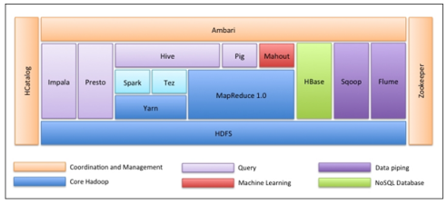
Hadoop has grown into a huge system. As long as it can be seen in fields related to massive data, the following are various data tools in Hadoop ecosystem.
(1)Data capture system: Nutch
(2)How to store massive data, of course, is a distributed file system: HDFS
(3)How to use the data? Analyze and process it
(4)MapReduce Framework allows you to write code to analyze big data
(5)Unstructured data (log) collection and processing: fuse/webdav/chukwa/flume/Scribe
(6)Import data to HDFS In, so far RDBSM You can also join HDFS: Hiho,sqoop
(7)MapReduce It's too troublesome for you to operate in a familiar way Hadoop Data in: Pig,Hive,Jaql
(8)Make your data visible: drilldown,Intellicus
(9)Manage your task flow in a high-level language: oozie,Cascading
(10)Hadoop Of course, it also has its own monitoring and management tools: Hue,karmasphere,eclipse plugin,cacti,ganglia
(11)Data serialization processing and task scheduling: Avro,Zookeeper
(12)More built on Hadoop Upper level services: Mahout,Elastic map Reduce
(13)OLTP Online transaction processing system: Hbase
The overall ecological map of Apache Hadoop is as follows.
In short, Hadoop is currently the preferred tool for analyzing massive data, and has been widely used in the following scenarios by all walks of life:
(1)Large data storage: distributed storage (various cloud disks, Baidu, 360)~There are also cloud platforms Hadoop Application)
(2)Log processing: Hadoop Good at this
(3)Mass Computing: Parallel Computing
(4)ETL: Data extraction to oracle,mysql,DB2,mongdb And mainstream database
(5)use HBase Do data analysis: deal with a large number of read and write operations with scalability - Facebook Based on HBase Real time data analysis system based on
(6)Machine learning: for example Apache Mahout Project( Apache Mahout Introduction (common fields: collaborative screening, clustering and classification)
(7)Search Engines: Hadoop + lucene realization
(8)Data mining: a popular advertising recommendation
(9)User behavior feature modeling
(10)Personalized advertising recommendation
2, The role of big data in Hadoop
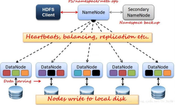
Hadoop is an open source distributed storage and computing platform. Among them, Hdfs is a distributed file storage system, which is used to store files. There are three roles involved in the storage system.
1. NameNode: manages metadata information and assigns tasks to child nodes (FSImage is the snapshot of the entire file system (metadata image file) when the primary node starts, and Edits is the modification record (operation log file))
2. DataNode: responsible for data storage and reporting heartbeat to the master node in real time
3,SecondaryNameNode:
1) First, it periodically goes to the NameNode to obtain edit logs and updates them to the fsimage. Once it has a new fsimage file, it copies it back to the NameNode.
2) This file will take less time to restart the fsname next time.
These three roles determine the operation architecture of hadoop distributed file system hdfs, as shown in the figure below.
yarnYarn, the framework of mapreduce for distributed computing, is a resource management system with the following roles.
1. The resource manager monitors the NodeManager and is responsible for the resource scheduling of the cluster
2. nodemanager manages node resources and processes ResourceManager commands
3, Construction of Hadoop platform environment
Hadoop runs on Linux. Although it can also run on Windows with the help of tools, it is recommended to run on Linux system. Here we first introduce the installation, configuration and Java JDK installation of Linux environment.
1. Installation of Linux Environment
Here, use Vmware virtual machine to install Linux. First, you need to set the Vmware virtual machine and host to NAT mode configuration. Nat is network address translation. It adds an address translation service between the host and the virtual machine, which is responsible for the communication transfer and IP conversion between the external and the virtual machine.
(1) After Vmware is installed, the default NAT settings are as follows:
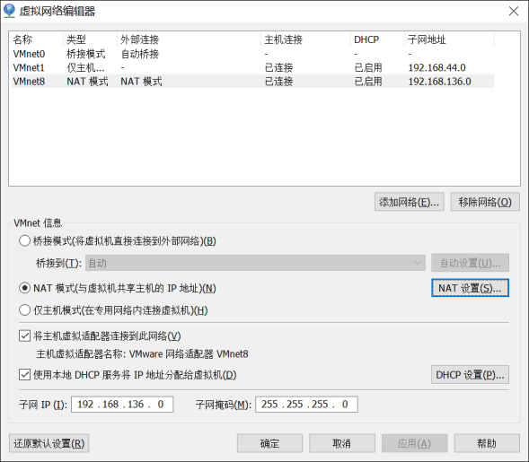
(2) The default setting is to start the DHCP service. NAT will automatically assign IP to the virtual machine. You need to fix the IP of each machine, so you need to cancel this default setting.
(3) Set a subnet segment for the machine. The default is 192.168.136. Here, set it as 100. In the future, the Ip of each virtual machine will be 192.168.100. *.
(4) Click the NAT setting button to open the dialog box, where you can modify the gateway address and DNS address. Specify the DNS address for NAT here.
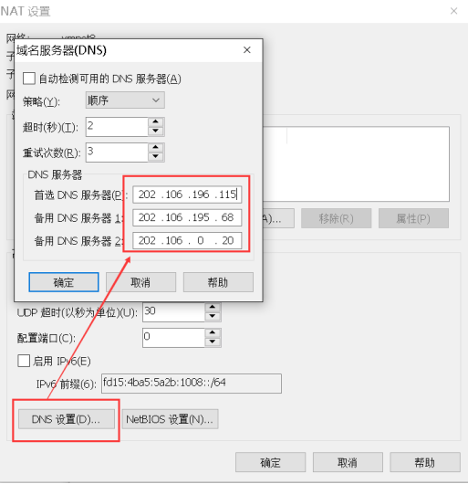
(5) The gateway address is the. 2 address in the current network segment. It is fixed here and will not be modified. Just remember the gateway address first, which will be used later.
2. Installation of Linux Environment
(1) Select new virtual machine from the file menu
(2) Select the classic type to install. Next.
(3) Choose to install the operating system later. Next.
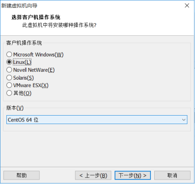
(4) Select Linux system and CentOS 64 bit version.
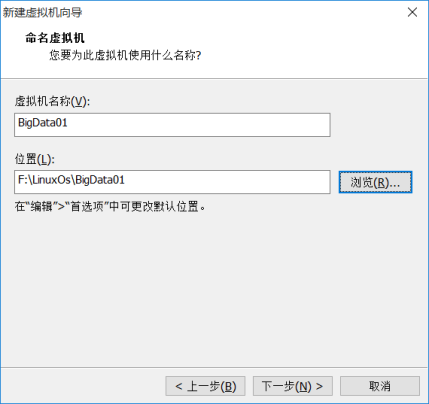
(5) Name the virtual machine and give it a name, which will be displayed on the left side of Vmware in the future. And select the directory where the Linux system is saved in the host. One virtual machine should be saved in one directory, and multiple virtual machines cannot use one directory.
(6) The specified disk capacity is the size of the hard disk allocated to the Linux virtual machine. It can be 20G by default. Next step.
(7) Click Customize hardware to view and modify the hardware configuration of the virtual machine. We don't modify it here.
(8) Click Finish to create a virtual machine, but the virtual machine is still an empty shell without an operating system. Next, install the operating system.
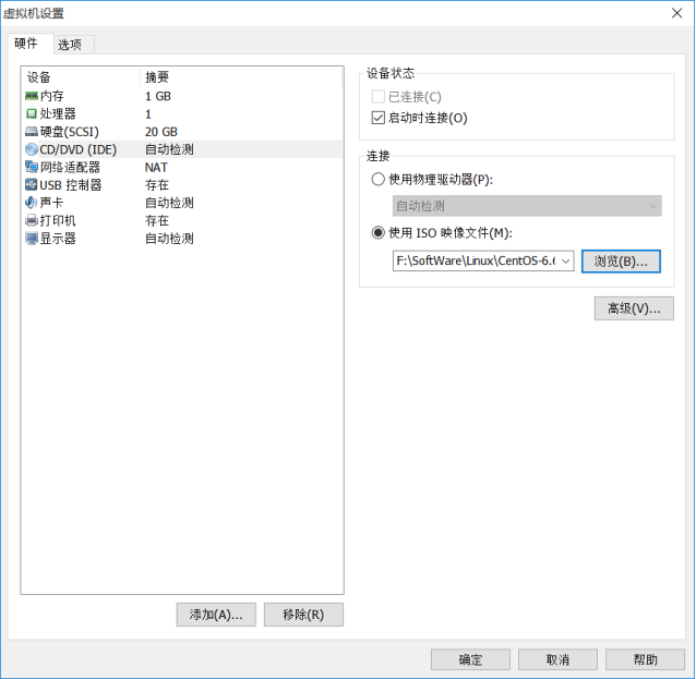
(9) Click Edit virtual machine settings, find the DVD, and specify the location of the operating system ISO file.
(10) Click to start this virtual machine, select the first enter to start installing the operating system.

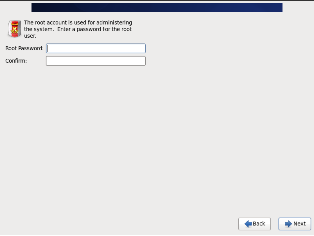
(11) Set the root password.
(12) Select Desktop, which will install an Xwindow.
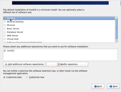
(13) First, do not add ordinary users, others use the default, and then install Linux.
3. Set up network
Because the DHCP automatic IP assignment function is turned off in the NAT setting of Vmware, Linux does not have IP yet. We need to set various network parameters.
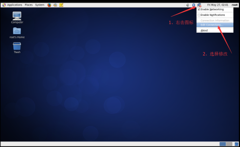
(1) Enter Xwindow with root, right-click the network connection icon in the upper right corner, and select Modify connection.
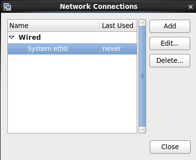
(2) The network connection lists all the network cards in the current Linux. There is only one network card System eth0 here. Click Edit.
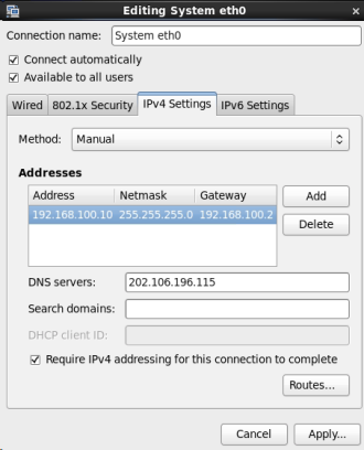
(3) Configure IP, subnet mask, gateway (the same as NAT settings), DNS and other parameters, because the network segment is set to 100. * in NAT, Therefore, this machine can be set to 192.168.100.10. The gateway is consistent with NAT, which is 192.168.100.2.
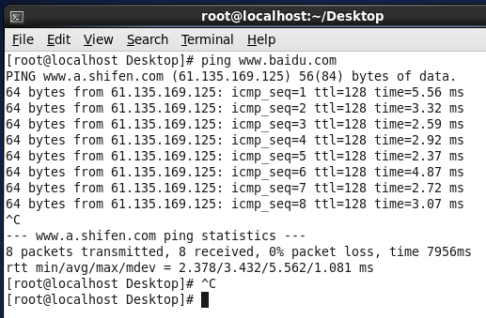
(4) Use ping to check whether you can connect to the external network. As shown in the figure below, the connection has been successful.
4. Modify hostname
To temporarily modify the hostname, you need to use the following instructions under linux.
[root@localhost Desktop]# hostname mylinux-virtual-machine
To permanently modify the hostname, you need to modify the configuration file / etc/sysconfig/network.
[root@mylinux-virtual-machine ~] vi /etc/sysconfig/network
After opening the file, make the following settings:
NETWORKING=yes  #Use network
HOSTNAME=mylinux-virtual-machine  #Host name setting
5. Turn off the firewall
The learning environment can turn off the firewall directly.
After logging in as root, execute to view the firewall status.
[root@mylinux-virtual-machine]#service iptables status
In some versions, the default firewall is firewall or ufw.
You can use temporary shutdown to turn off the firewall. The command is as follows.
[root@mylinux-virtual-machine]# service iptables stop
You can also permanently turn off the firewall with the following commands.
[root@mylinux-virtual-machine]# chkconfig iptables off
Turn off the firewall. This setting needs to be restarted to take effect.
selinux is a sub security mechanism of Linux, which can be disabled by the learning environment.
Disable selinux to edit the / etc/sysconfig/selinux file. The command to open the configuration file / etc/sysconfig/selinu is as follows.
[hadoop@mylinux-virtual-machine]$ vim /etc/sysconfig/selinux
Set selinux to disabled in the / etc/sysconfig/selinux file, as follows.
# This file controls the state of SELinux on the system.
# SELINUX= can take one of these three values:
#     enforcing - SELinux security policy is enforced.
#     permissive - SELinux prints warnings instead of enforcing.
#     disabled - No SELinux policy is loaded.
SELINUX=disabled
# SELINUXTYPE= can take one of these two values:
#     targeted - Targeted processes are protected,
#     mls - Multi Level Security protection.
SELINUXTYPE=targeted
6. Install Java JDK
Because the bottom layer of Hadoop is implemented in Java, you need to check whether Java has been installed in the environment.
Check whether java JDK has been installed. You can execute commands under linux.
[root@mylinux-virtual-machine /]# java –version
Note: the JDK on Hadoop machine is preferably the Java JDK of Oracle, otherwise there will be some problems, for example, there may be no JPS command.
If another version of JDK is installed, uninstall it.
You can download java version 8.0 or above from Oracle's official website. As shown in the figure below.
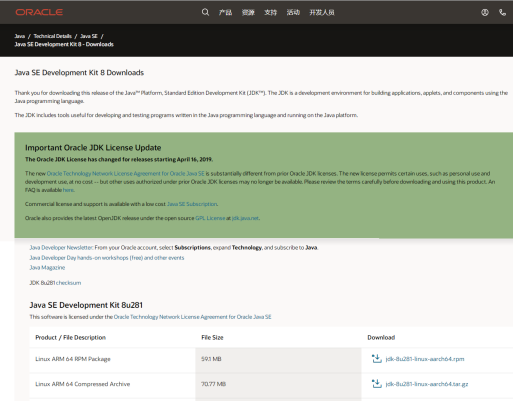
In the figure above, you can download the gz compressed package and decompress it under linux. For example, unzip it to the / usr/java directory. The usr directory exists in the linux system itself. The java directory can be created under the usr directory by itself. The commands for creating the usr directory under linux are as follows.
[root@mylinux-virtual-machine /]# tar -zxvf jdk-8u281-linux-x64.tar.gz -C /usr/java
Next, add environment variables.
Set the JDK environment variable JAVA_HOME. The configuration file / etc/profile needs to be modified. The modification commands in linux are as follows.
[root@mylinux-virtual-machine hadoop]#vi /etc/profile
After entering the file, add the following contents at the end of the file
export JAVA_HOME="/usr/java/jdk1.8.0_281"
export PATH=$JAVA_HOME/bin:$PATH
After modification, execute source /etc/profile
After installation, execute java – version again, and you can see that the installation has been completed.
[root@mylinux-virtual-machine /]# java -version
java version "1.7.0_67"
Java(TM) SE Runtime Environment (build 1.7.0_67-b01)
Java HotSpot(TM) 64-Bit Server VM (build 24.65-b04, mixed mode)
7. Hadoop local mode installation
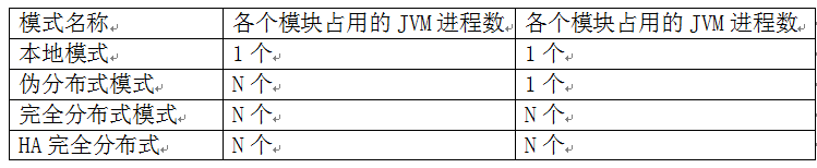
Hadoop deployment modes include: local mode, pseudo distributed mode, fully distributed mode and HA fully distributed mode.
The distinction is based on the NameNode, DataNode, ResourceManager, NodeManager and other modules running in several JVM processes and several machines.
Local mode is the simplest mode. All modules run in a JVM process and use the local file system instead of HDFS. Local mode is mainly used for running debugging in the local development process. After downloading the hadoop installation package, you don't need any settings. The default mode is local mode.
The hadoop installation package can be downloaded from the official website. As shown in the figure below.
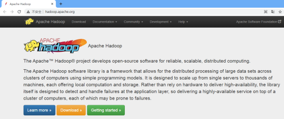
Click the "Download" button from the official website. Select the appropriate version to Download according to the needs, and decompress the compressed package in the linux environment after downloading. The linux commands are as follows.
[hadoop@mylinux-virtual-machine hadoop]# tar -zxvf hadoop-2.7.0.tar.gz -C /usr/hadoop
After decompression, configure the Hadoop environment variable, and modify the / etc/profile command under linux as follows.
[hadoop@mylinux-virtual-machine hadoop]# vi /etc/profile
Add the following configuration information to the profile file.
export HADOOP_HOME="/opt/modules/hadoop-2.5.0"
export PATH=$HADOOP_HOME/bin:$HADOOP_HOME/sbin:$PATH
Execute: source /etc/profile makes the configuration effective
Next, enter the etc/hadoop directory under the extracted directory and set the five files.
Step 1: set Hadoop env SH file, modify Java in configuration information_ The home parameters are as follows.
export JAVA_HOME="/usr/java/jdk1.8.0_281"
Step 2: modify and configure the core site XML file. The amendments are as follows.
<configuration>
    <property>
        <name>fs.defaultFS</name>
        <value>hdfs://mylinux-virtual-machine:9000</value>
    </property>
    <property>
        <name>hadoop.tmp.dir</name>
        <value>/opt/data/tmp</value>
    </property>
</configuration>
fs. The defaultfs parameter configures the address of HDFS. hadoop.tmp.dir configures the Hadoop temporary directory.
Step 2: modify the configuration of HDFS site XML file. The amendments are as follows.
<configuration>
    <property>
        <name>dfs.replication</name>
        <value>1</value>
    </property>
</configuration>
dfs.replication configures the number of backups during HDFS storage. Because this is a pseudo distributed environment with only one node, it is set to 1.
Step 4 configure mapred site xml
There is no mapred site by default XML file, but there is a mapred site xml. Template configuration template file. Copy the template to generate mapred site xml. The copy command is as follows.
[hadoop@mylinux-virtual-machine hadoop]#cp etc/hadoop/mapred-site.xml.template etc/hadoop/mapred-site.xml
At mapred site Add the following configuration to XML.
<property>
    <name>mapreduce.framework.name</name>
    <value>yarn</value>
</property>
This configuration is used to specify that mapreduce runs on the yarn framework.
Step 5 configure yen site xml
At yarn site Add configuration information to XML as follows.
<configuration>
    <property>
        <name>yarn.nodemanager.aux-services</name>
        <value>mapreduce_shuffle</value>
    </property>
    <property>
        <name>yarn.resourcemanager.hostname</name>
        <value>mylinux-virtual-machine</value>
    </property>
</configuration>
yarn. nodemanager. Aux services configures the default shuffling method of yarn and selects the default shuffling algorithm of mapreduce.
yarn.resourcemanager.hostname specifies the node on which the resource manager runs.
After the configuration file information in these five steps is configured successfully, format HDFS. The instructions for formatting HDFS in linux system are as follows.
hdfs namenode -format
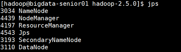
After executing the command, you will be asked to enter the password three times during service startup. After execution, make jps display process information, as shown in the following figure.
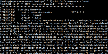
If you find the "has Successful" information in this message, it proves that the hadoop format has been successful.
Formatting is to block the DataNode in the distributed file system HDFS, and count the initial metadata after all blocks and store it in the NameNode.
After formatting, check the core site Hadoop.xml tmp. Whether there is a dfs directory under the directory specified by dir (in this case, / opt/data directory). If so, it indicates that the format is successful.
To start hadoop platform, you can start hdfs first. The execution path of the command is in the / sbin directory in the extracted hadoop path. The specific startup method is executed in linux as follows.
[hadoop@mylinux-virtual-machine sbin]#./start-dfs.sh
The execution result is shown in the figure.
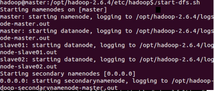
After starting hdfs, you can use jsp to view the process, as shown in the figure.
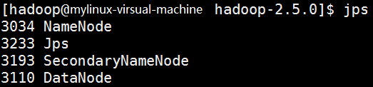
As can be seen from the figure, NameNode, SecondNameNode and DataNode have been started in the process.
Next, continue to start the yarn framework. The startup directory is still under the / sbin directory in the extracted hadoop path. The specific startup method is executed in linux as follows.
[hadoop@mylinux-virtual-machine sbin]#./start-yarn.sh
The execution result is shown in the figure.
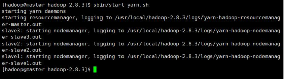
After the yarn service is started, continue to use jps to view the process information, as shown in the following figure.
So far, the Hadoop environment has been built.
3, Construction of Spark platform environment
It is the most effective data processing framework in today's enterprises. Using Spark is expensive because it requires a lot of memory for calculation, but it is still a favorite of data scientists and big data engineers.
To download spark compressed package, you need to visit Spark's official website.
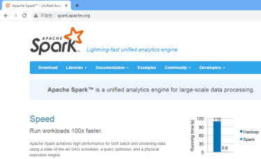
After entering the website, select the "Download" option to Download the specified version.
After downloading, unzip it on the linux platform and unzip it to the spark custom directory under the usr directory. The linux commands are as follows.
[hadoop@mylinux-virtual-machine hadoop]# tar -zxvf spark-3.1.1-bin-hadoop2.7.tgz -C /usr/spark
Next, open the Spark configuration directory and copy the default Spark environment template. It has been published as Spark env The form of sh.template appears. Use the cp command to copy a copy and remove ". Template" from the generated copy. The linux commands are as follows.
[hadoop@mylinux-virtual-machine sbin]#cd /usr/lib/spark/conf/
[hadoop@mylinux-virtual-machine conf]#cp spark-env.sh.template spark-env.sh
[hadoop@mylinux-virtual-machine conf]# vi spark-env.sh
Add information to file
export JAVA_HOME=/usr/java/jdk1.8.0_281
export HADOOP_HOME=/usr/hadoop/hadoop-2.7.0
export PYSPARK_PYTHON=/usr/bin/python3
In the configuration information, JAVAHOME and hadoop are path variables of java and hadoop, PYSPARK_PYTHON is the variable information that Python contacts with pyspark, / usr/bin/python is the path of python3 in linux. You can find out whether you can find python3 through such path operation.
5, Classic big data wordCount program
To understand the big data platform, we need to conduct data analysis on the big data platform. The data analysis process of the big data platform is shown in the figure below.
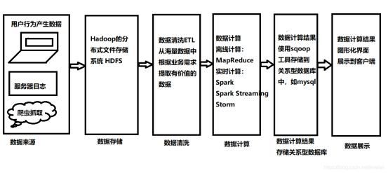
The most important program in the analysis process shown in the figure is the WordCount program. The WordCount program comes entirely from the idea of MapReduce's distributed computing. Let's first explain the calculation idea of MapReduce.
First look at the following figure.
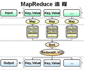
It can be seen from the process that MapReduce has two stages. In the Map stage, the slices of the input big data file are first processed into the form of key value pairs, and then the Map task is called for each value pair, which is processed into new key value pairs through the Map task. Most of the analysis ideas of data analysis are grouping, sorting, summarizing and statistics. The reduce phase of MapReduce is also a grouping, sorting, summary and statistics phase. Finally, it is output as a data set of value pairs.
For the WordCount program, that is to count the number of words in the distributed file system. Its input content and output format are shown in the figure below.

As can be seen from the figure, each sentence composed of English words in the input file is finally processed through the MapReduce process, and the number of occurrences of each word in the file is output.
The idea of using MapReduce process to process such wordCount program is shown in the figure below.
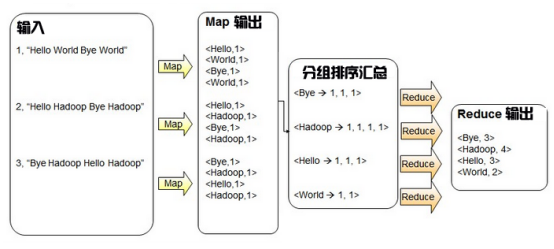
It can be seen from the figure that the input is a sentence containing English words in each line. After the Map process, it becomes a value pair of English words and counting formula. This key value format is only for counting numbers. "< Hello, 1 >" means that there is one "hello". Later in the counting process, there will be "< Hello, 1 >" and one "hello", This only needs to segment the English sentence according to the space, and construct the format of (Hello, 1) for each word. The output results after the Map process are grouped in the form of key, that is, grouping with "hello" as the key, and the subsequent data are summarized, counted and summed. Finally, the output results after summary statistics are generated through the Reduce process.
Here's the code.
The Spark conversation of SparkSession must be instantiated when using PySpark. The specific instantiation format is as follows.
SparkSession.builder.master("local").appName("wordCount").getOrCreate()
Builder refers to that SparkSession is instantiated through the static class builder. After calling the builder, you can call many methods in the builder static class.
The master function sets the Spark master URL connection. For example, "local" is set to run locally, "local[4]" runs 4cores locally, or“ spark://master:7077 "Run in the spark standalone cluster.
The appName(String name) function is used to set the application name, which will be displayed in Spark web UI.
getOrCreate() gets the obtained SparkSession, or if it does not exist, creates a new SparkSession based on the builder option.
After the SparkSession dialog is established, sparkcontext is the first class used to write spark programs. Sparkcontext is the main entry point of Spark Program, so after SparkSession establishes a dialogue, obtain the dialogue variable sparkcontext program. The specific codes are as follows:
from pyspark.sql import SparkSession
spark=SparkSession.builder.master("local").appName("wordCount").getOrCreate()
sc=spark.sparkContext
With sparkContext, the entry of Spark Program, to complete the work of data analysis, we must first read the file to be analyzed and load a file to create RDD. RDD is the most basic data abstraction in spark. RDD (Resilient Distributed Dataset) is called elastic distributed dataset, which represents an immutable, divisible and parallel computing set of elements. Spark has a collect method, which can convert RDD type data into an array for display. If you want to display the read RDD data, you can use textFile to read the data in hdfs, and then display it through the collect method. textFile reads the file from hdfs by default, or you can specify sc.textFile("path") Adding hdfs: / / before the path indicates reading data from the hdfs file system. The specific code is as follows.
from pyspark.sql import SparkSession
spark=SparkSession.builder.master("local").appName("wordCount").getOrCreate()
sc=spark.sparkContext
files=sc.textFile("hdfs://mylinux-virtual-machine:9000/words.txt")
print(files.collect())
In the code, read the words on the hdfs server through textFile Txt file. After reading, it is RDD type data through files The collect () method is converted into an array and printed by the print method. The operation results are as follows.
It can be seen from the results in the figure that the data in the file has been read out and formed a list. By traversing the read RDD, you can operate on each data in the RDD.
There are two very important functions in spark: map function and flatMap function, which are two commonly used functions. among
map: Operate on each element in the collection.
flatMap: Each element in the collection is manipulated and then flattened.
If you use the collect() method to display the specific contents of the RDD read earlier through the map operation, the code is as follows.
from pyspark.sql import SparkSession
spark=SparkSession.builder.master("local").appName("wordCount").getOrCreate()
sc=spark.sparkContext
files=sc.textFile("hdfs://mylinux-virtual-machine:9000/words.txt")
map_files=files.map(lambda x:x.split(" "))
print(map_files)
The operation results are as follows:

If you use the flatMap operation to read the RDD before, and then use the collect() method to display the specific content, the code is as follows.
from pyspark.sql import SparkSession
spark=SparkSession.builder.master("local").appName("wordCount").getOrCreate()
sc=spark.sparkContext
files=sc.textFile("hdfs://mylinux-virtual-machine:9000/words.txt")
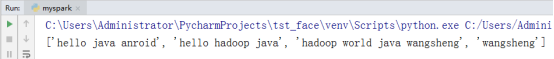
flatmap_files=files.flatMap(lambda x:x.split(" "))
print(flatmap_files)
The operation results are as follows:

According to the returned result sets of two different operations on each element: map and flatMap, it can be seen that the returned result of flatMap is more in line with the expectation for the problem of wordCount. Then process the result set returned by flatMap to form (hello, 1), (java, 1), (android, 1) and other forms in the form of counting key value pairs. The code is as follows.
from pyspark.sql import SparkSession
spark=SparkSession.builder.master("local").appName("wordCount").getOrCreate()
sc=spark.sparkContext
files=sc.textFile("hdfs://mylinux-virtual-machine:9000/words.txt")
flatmap_files=files.flatMap(lambda x:x.split(" "))
map_files=flatmap_files.map(lambda x:(x,1))
print(map_files.collect())
The operation results are as follows.

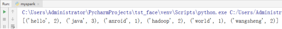
After constructing the key Value data as shown in the above figure, use the reduceByKey method in spark. reduceByKey is to perform a function reduce operation on the Value of the element with the same key in the RDD whose element is a KV pair. Therefore, the values of multiple elements with the same key are reduced to a Value, and then form a new KV pair with the key in the original RDD. What is implemented here is the summation of the values corresponding to the same key, which can be completed by lambda function. The code is as follows.
from pyspark.sql import SparkSession
spark=SparkSession.builder.master("local").appName("wordCount").getOrCreate()
sc=spark.sparkContext
files=sc.textFile("hdfs://mylinux-virtual-machine:9000/words.txt")
flatmap_files=files.flatMap(lambda x:x.split(" "))
map_files=flatmap_files.map(lambda x:(x,1))
freduce_map=map_files.reduceByKey(lambda x,y:x+y)
print(reduce_map.collct())
The final output of the program is shown in the figure.
Video Explanation address:
1. pyspark analysis big data 1-hadoop environment construction: https://www.bilibili.com/video/BV1Z54y1L7cT/
2. pyspark analysis big data 2-mapreduce process: https://www.bilibili.com/video/BV15V411J75a/
3. Pyspark analysis big data 3-pyspark analysis wordcount program and extension: https://www.bilibili.com/video/BV1y64y1m7XN/