1. Data loading
PyTorch has developed standard conventions for interacting with data, so it can process data consistently, regardless of image, text or audio. The two main conventions for interacting with data are dataset and data loader. Dataset is a Python class that enables us to obtain the data provided to neural networks. The data loader provides data from the data set to the network.
PyTorch through torch utils. Data encapsulates the commonly used data loading, which can easily realize multi-threaded data pre reading and batch loading. In addition, torchvision has implemented common image data sets in advance, including CIFAR-10, ImageNet, COCO, MNIST, LSUN and other data sets previously used, which can be accessed through torchvision Datasets are convenient to call.
1.1,Dataset
Dataset is an abstract class. In order to facilitate reading, you need to wrap the data to be used as dataset class. A custom dataset needs to inherit it and implement two member methods:
- __ getitem__ () this method defines to obtain a piece of data or a sample with indexes (0 to len(self)).
- __ len__ () this method returns the total length of the dataset.
from torch.utils.data import Dataset
import pandas as pd

# Define a dataset
class BulldozerDataset(Dataset):
    """ Dataset presentation """
    def __init__(self, csv_file):
        """Implement the initialization method to read and load data during initialization"""
        self.df = pd.read_csv(csv_file)
    def __len__(self):
        '''
        return df Length of
        '''
        return len(self.df)
    def __getitem__(self, idx):
        '''
        according to idx Return a row of data
        '''
        return self.df.iloc[idx].Title
if __name__ == '__main__':
    ds_demo = BulldozerDataset('Highest Holywood Grossing Movies.csv')
    print(len(ds_demo))
    print(ds_demo[0])
=================================================
918
Star Wars: Episode VII - The Force Awakens (2015)
1.2,Dataloader
DataLoader provides us with the operation of reading datasets. The common parameters are:
- dataset(Dataset): the incoming dataset.
- batch_size: the size of each batch.
- shuffle: reorder the data at the beginning of each epoch.
- num_workers: several sub processes are used when loading data. The thread parameter under windows is set to 0, which is safe.
dl = torch.utils.data.DataLoader(ds_demo, batch_size=10, shuffle=True, num_workers=0)
The DataLoader returns an iteratable object. We can use the iterator to obtain data in stages:
idata=iter(dl)
print(next(idata))
====================
['Cars 3 (2017)', 'Dick Tracy (1990)', 'Click (2006)', 'Star Trek: The Motion Picture (1979)', 'Apocalypse Now (1979)', 'The Devil Wears Prada (2006)', 'The Divergent Series: Insurgent (2015)', 'As Good as It Gets (1997)', 'Safe House (2012)', 'Puss in Boots (2011)']
The common usage is to use the for loop to traverse it:
ds_demo = BulldozerDataset('Highest Holywood Grossing Movies.csv')
    dl = torch.utils.data.DataLoader(ds_demo, batch_size=10, shuffle=True, num_workers=0)
    for i, data in enumerate(dl):
        print(i, data)
===================================
0 ['Catch Me If You Can (2002)', 'Cast Away (2000)', "Miss Peregrine's Home for Peculiar Children (2016)", 'Django Unchained (2012)', 'xXx (2002)', 'Iron Man 2 (2010)', 'The Meg (2018)', 'Despicable Me 2 (2013)', 'Peter Rabbit (2018)', 'Bridesmaids (2011)']
...
1.3,torchvision
torchvision is a library dedicated to image processing in PyTorch Datasets can be understood as datasets customized by PyTorch team. These datasets help us deal with a lot of image datasets in advance. We can use them directly: - MNIST - COCO - Captions - Detection - LSUN - ImageFolder - Imagenet-12 - CIFAR - STL10 - SVHN - PhotoTour. We can use them directly.
Torchvision installation: pip install torchvision.
import torchvision.datasets as datasets
trainset = datasets.CIFAR10(root='./data', # Indicates the directory where MNIST data is loaded
                            train=True,  # Indicates whether to load the training set of the database. If false, load the test set
                            download=True, # Indicates whether MNIST datasets are automatically downloaded
                            transform=None) # Indicates whether data preprocessing is required. none indicates no preprocessing
torchvision.models: torchvision not only provides common image data sets, but also provides trained models, which can be loaded and used directly, or in the process of migration and learning torchvision The sub modules of the models module contain the following model structures- AlexNet - VGG - ResNet - SqueezeNet - DenseNet.
#We can directly use the trained model. Of course, this is the same as datasets, which need to be downloaded from the server
import torchvision.models as models
resnet18 = models.resnet18(pretrained=True)#True: load the model and set it to pre training mode
torchvision.transforms: the transforms module provides general image conversion operation classes for data processing and data enhancement.
rom torchvision import transforms as transforms
transform = transforms.Compose([
    transforms.RandomCrop(32, padding=4),  #Fill 0 around first, and then cut the image randomly into 32 * 32
    transforms.RandomHorizontalFlip(),  #Half the probability of image flipping, half the probability of not flipping
    transforms.RandomRotation((-45,45)), #Random rotation
    transforms.ToTensor(),
    transforms.Normalize((0.4914, 0.4822, 0.4465), (0.229, 0.224, 0.225)), #R. Mean and variance used for normalization of each layer of G and B
])
(0.485, 0.456, 0.406), (0.2023, 0.1994, 0.2010): according to the normalization parameters of ImageNet training, it can be used directly. It can be considered as a fixed value, or other values can be used.
2. Mathematical principles
2.1, loss function
Loss function is used to estimate the inconsistency between the predicted value (output in our example) and the real value (y_train in our example). It is a non negative real value function. The smaller the loss function, the better the robustness of the model. The process of training the model is to make the loss function smaller and smaller through continuous iterative calculation and gradient descent optimization algorithm. The smaller the loss function is, the better the algorithm is.
Machine Learning: Concepts_ Yan Shuangying CSDN blog 1, overview of Machine Learning 1.1, the concept of Machine Learning, Machine Learning, that is, Machine Learning, involves probability theory, statistics, approximation theory, convex analysis, algorithm complexity theory and other disciplines. The purpose is to let the computer simulate or realize human learning behavior, so as to obtain new knowledge or skills, reorganize the existing knowledge structure and constantly improve its own performance. In short, Machine Learning is that people train machines by providing a large amount of relevant data. DataAnalysis: basic concepts, environment introduction, environment construction, big data problems_ Yan Shuangying CSDN blog 1, overview 1.1, the nature of data. The so-called data is the symbol describing things, which records the nature, state and relationship of objective things https://shao12138.blog.csdn.net/article/details/120507206#t8 Because PyTorch is calculated using mini batch, the calculation result of loss function has averaged Mini batch.
-
nn.L1Loss (sum square error): enter the absolute value of the difference between x and target y. it is required that the dimensions of x and y should be the same (can be vector or matrix), and the resulting loss dimension also corresponds to the same.
-
nn.NLLLoss: negative log likelihood loss function for multi classification.
-
nn.CrossEntropyLoss: cross entropy loss function for multi classification.
-
nn.BCELoss: calculate the binary cross entropy between x and y.
2.2 gradient descent
In calculus, we find the parameters of multivariate functions Partial derivative, the partial derivative of each parameter obtained is written in the form of vector, which is the gradient. For example, function
  , respectively
 To find the partial derivative, the gradient vector is
  , abbreviation
 perhaps
  .
.
Geometrically speaking, the gradient is where the function changes and increases the fastest. It is easier to find the maximum value of the function along the direction of the gradient vector. Conversely, the gradient decreases the fastest in the opposite direction of the gradient vector, that is, it is easier to find the minimum value of the function.
We need to minimize the loss function, which can be solved step by step iteratively through the gradient descent method to obtain the minimized loss function and the value of model parameters.
Visual explanation of gradient descent method: gradient descent method is like going down the mountain. We don't know the way down the mountain, so we decide to take one step at a time. When we reach a position, we solve the gradient of the current position, take a step down along the negative direction of the gradient, that is, the steepest position at present, and then continue to solve the gradient of the current position, Take a step to the position where this step is located and follow the steepest and most downhill position. Go on like this step by step until we feel that we have reached the foot of the mountain.
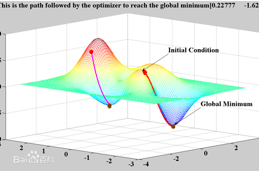
If we go on like this, we may not be able to go to the foot of the mountain, but to the lower part of a local peak (local optimal solution).
This problem may be encountered in previous machine learning, because there are few features in machine learning, so it is likely to fall into a local optimal solution, but in deep learning, there are millions or even hundreds of millions of features, and the probability of this situation is almost zero, so we don't need to consider this problem.
2.3 gradient descent method of mini batch
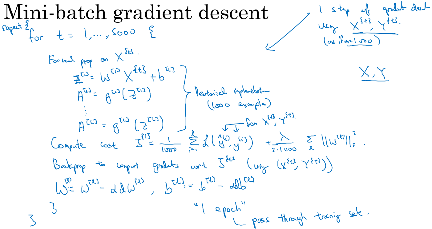
When performing gradient descent method on the whole training set, the whole training data set must be processed before one-step gradient descent, that is, each step of gradient descent method needs to process the whole training set once. If the training data set is large, the processing speed will be very slow, and it is impossible to load it into memory or video memory at one time, Therefore, we will divide the large data set into small data sets and train part by part. This training subset is called mini batch.
This method is used for training in PyTorch. You can see batch in the introduction to dataloader_ Size is the size of our mini batch.
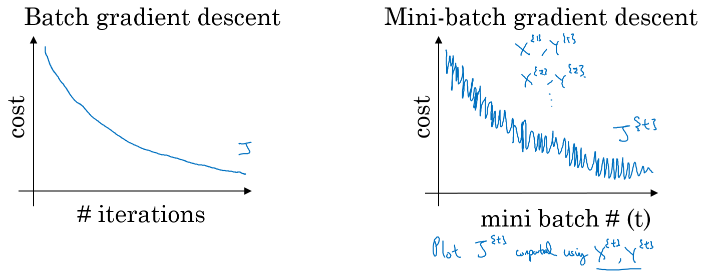
For the ordinary gradient descent method, an epoch can only perform gradient descent once; For the mini batch gradient descent method, an epoch can perform several gradient descent of mini batch.
The change trend of cost function of ordinary batch gradient descent method and mini batch gradient descent method is shown in the following figure:
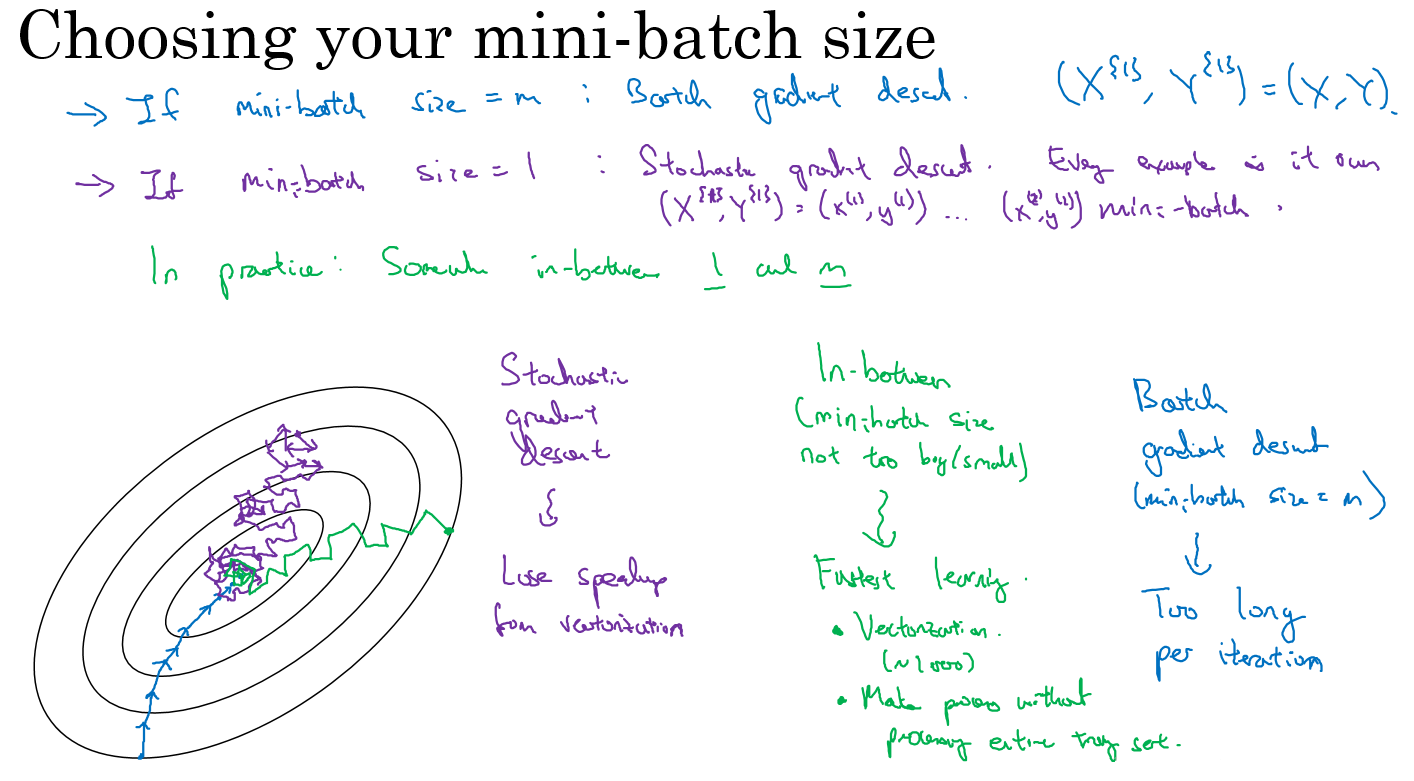
- if the size of training samples is relatively small and can be read into memory at one time, we don't need to use mini batch.
- if the size of the training sample is relatively large and cannot be read into the memory or existing at one time, we must use mini batch to calculate in batches - the calculation rules of mini batch size are as follows, and the size to the nth power of 2 is used when the maximum memory is allowed.
torch.optim is a library that implements various optimization algorithms. Most commonly used optimization algorithms have been implemented. We can call them directly.
torch.optim.SGD
Random gradient descent algorithm. The algorithm with momentum can be set as an optional parameter. The example is as follows:
#lr parameter is the learning rate. For SGD, 0.1 0.01.0.001 is generally selected. How to set it will be described in detail in the later practical chapter
##If momentum is set, it is SGD with momentum, which can not be set
optimizer = torch.optim.SGD(model.parameters(), lr=0.1, momentum=0.9)
torch.optim.RMSprop
In addition to the above Momentum gradient descent method, RMSprop (root mean square prop) is also an algorithm that can speed up the gradient descent. Using RMSprop algorithm, we can reduce the large fluctuation of gradient update in some dimensions and make the gradient descent faster.
#RMSprop will not be used in our course, so only one example is given here
optimizer = torch.optim.RMSprop(model.parameters(), lr=0.01, alpha=0.99)
torch.optim.Adam
The basic idea of Adam optimization algorithm is to combine Momentum and RMSprop to form an optimization algorithm suitable for different deep learning structures.
# lr, betas, and eps here all use default values, so Adam is the simplest optimization method to use
optimizer = torch.optim.Adam(model.parameters(), lr=0.001, betas=(0.9, 0.999), eps=1e-08)
2.4, variance & deviation
The deviation measures the deviation between the expected prediction of the learning algorithm and the real result, and immediately draws the fitting ability of the learning algorithm itself.
Variance measures the change of learning performance caused by the change of the training set of the same size, that is, the generalization ability of the model.

high bias: it is generally called underfitting, that is, our model does not adapt well to the existing data, and the degree of fitting is not enough.
high variance: it is generally called overfitting, that is, the fitting degree of the model to the training data is too high and the generalization ability is lost.
Under fitting solution:
- Increase the network structure, such as increasing the number of hidden layers;
- Train longer;
- Find a suitable network architecture and use a larger NN structure;
Over fitting solution:
- Use more data;
- regularization;
- Looking for a suitable network structure;
#Calculated deviation:
print (5-w.data.item(),7-b.data.item())
3. Cat fish image classification
3.1. Establish training set
Next, we need to convert them into a format that PyTorch can understand. There is a class named ImageFolder in the torchvision package, which can do everything for us. As long as our images are in an appropriate directory structure, each directory is a label (for example, all cats are in a directory named cat):
import torchvision
from torchvision import transforms

train_data_path = "/train/"
transforms = transforms.Compose([
    transforms.Resize(64),  #Scale each image to the same resolution 64 * 64
    transforms.ToTensor(),  #Convert the image into a tensor
    transforms.Normalize(mean=[0.485, 0.456, 0.406], std=[0.229, 0.224, 0.225]) #Normalize according to the specific mean value to get the super parameters.
])
train_data = torchvision.datasets.ImageFolder(root=train_data_path, transforms=transforms)
Adjust the image size to 64 * 64, which is adjusted at will, so that the next first network can calculate quickly. Generally speaking, most existing frameworks use 224 * 224 or 299 * 299 image input. The larger the input size, the more data the network learns, but usually the GPU memory can hold a small batch of images.
torchvision allows you to specify a list of transformations that can be applied before the image is input to the neural network. The default conversion is to convert the image into a tensor (transforms.ToTensor() method), and you can also do some work that may not seem obvious.
Normalization is important because a lot of multiplication is done when the input passes through the neural network layer; Ensuring that the incoming value is between 0 and 1 can prevent the median value in the training stage from becoming too large (gradient explosion). The magic parameters used here are the mean and standard deviation of the entire ImageNet dataset. You can specifically calculate the mean and standard deviation of the whole subset of fish and cats, but these parameters of ImageNet dataset are enough (if you deal with a completely different dataset, you must calculate the mean and standard deviation, and it is acceptable to use ImageNet constants directly).
3.2 establish verification set and test set
One danger of deep learning is over fitting: your model can really identify the trained data well, but it can't be generalized to examples it hasn't seen. When it sees an image of a cat, the model will not think of it as a cat, even though they are cats, unless the images of other cats are very similar to this image. In order to prevent this problem in the network, a verification set is prepared, which is a series of images of cats and fish that do not appear in the training set. At the end of each training cycle (epoch), we compare it with this verification set to ensure that our network does not make mistakes.
In addition to a verification set, you also need to create a test set, which will be used to test the model after all training is completed.
train_data_path = "/train/"
val_data_path = "/val/"
test_data_path = "/test/"
train_data = torchvision.datasets.ImageFolder(root=train_data_path, transforms=transforms)
val_data = torchvision.datasets.ImageFolder(root=val_data_path, transforms=transforms)
test_data = torchvision.datasets.ImageFolder(root=test_data_path, transforms=transforms)
To create a data loader:
import torchvision.datasets as data
batch_size = 64
train_data_loader = data.DataLoader(train_data, batch_size=batch_size)
val_data_loader = data.DataLoader(val_data, batch_size=batch_size)
test_data_loader = data.DataLoader(test_data, batch_size=batch_size)
batch_size: how many images will be provided to the network before training and updating the network. In theory, batch_size is set to the number of images in the test and training set, so that the network will see each image before updating. But in practice, we don't do this because smaller batches require less memory than storing all the relevant information of each image in the dataset, and smaller batches will make the training faster so that we can update the network faster.
PyTorch's data loader will batch_size is set to 1 by default, and you will almost certainly change this. You can also specify how the dataset is sampled, whether the dataset is disrupted at each run, and how many work processes are required to fetch data from the dataset.
3.3. Build neural network
Neural network structure: an input layer, which processes the input tensor (our image); Another output layer whose size is the number of output categories (2); A hidden layer between the two; Full connection is adopted between layers.
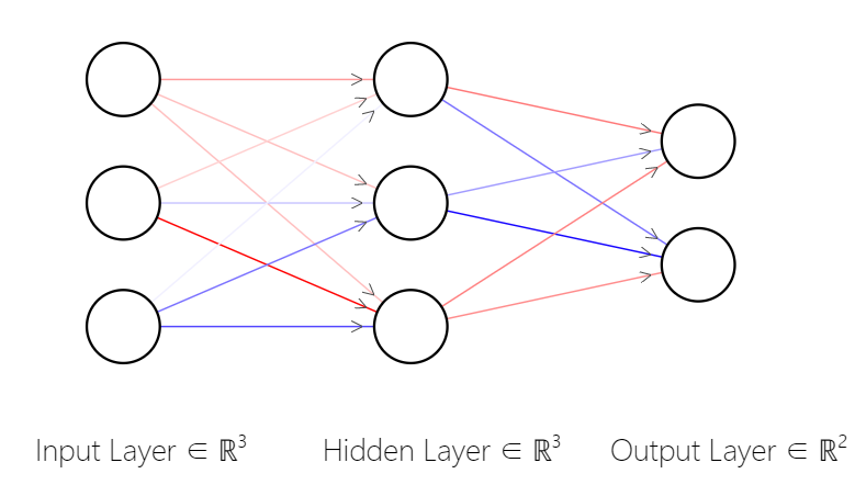
The neural network in the figure has an input layer with three nodes, a hidden layer with three nodes and an output layer with two nodes. It can be seen that in the full connection, each node will affect each node in the next layer, and each connection has a weight, which determines the strength of the signal from this node to the next layer (the main purpose of training is to update these weights, which usually starts with randomization). When an input is introduced into the network, the weight and the offset of this layer can be simply multiplied by the matrix.
To create a neural network in PyTorch, you need to inherit a named torch nn. Class of network, fill in__ init__ And forward methods:
import torch.nn as nn
import torch.nn.functional as F

class SimpleNet(nn.Module):
    def __init__(self):
        super(SimpleNet, self).__init__()
        #Establish 3 full connection layers
        self.fc1 = nn.Linear(12288, 84)
        self.fc2 = nn.Linear(84, 50)
        self.fc3 = nn.Linear(50, 2)
    def forward(self, x):
        #The three-dimensional vector in the image is converted into a one-dimensional vector, which can be input to the first fully connected layer
        x = x.view(-1, 12288)
        #Call activation function
        x = F.relu(self.fc1(x))
        x = F.relu(self.fc2(x))
        x = F.softmax(self.fc3(x))
        #Return the result of softmax activation function as the classification result
        return x
simplenet = SimpleNet()
The number of nodes in the hidden layer can be arbitrary, but the number of nodes in the final output layer is required to be 2, which corresponds to our classification results. Generally speaking, you want the data in the layer to be compressed when passing down. For example, if a layer has 50 inputs to 100 outputs, the network only needs to transfer 50 connections to 50 of the 100 outputs when learning, and it is considered that its work is completed. Reducing the size of the output according to the input can require this part of the network to learn a representation of the original input with less resources, which often means that it will extract some features in the image that are important to the problem we want to solve.
3.4, loss function and optimizer
Loss function is one of the key links of effective deep learning solution. PyTorch uses the loss function to determine how to update the network to achieve the desired results. According to your needs, the loss function can be complex or simple. PyTorch provides a complete set of loss functions, covering most applications you may encounter. Of course, you can also customize the loss function.
import torch.optim as optim
criterion = nn.CrossEntropyLoss()
optimizer = optim.Adam(simplenet.parameters(), lr=0.001)
One of the important improvements made by Adam (and RMSProp and AdaGrad) compared with SGD is to use a learning rate for each parameter and adjust the learning rate according to the change rate of these parameters. It will maintain a list of exponentially decaying gradients and the squares of these gradients, and use them to adjust the global learning rate used by Adam. According to experience, Adam is far better than most other optimizers for deep learning networks, but you can also replace Adam with SGD or RMSProp.
3.5 model training
def train(model, optimizer, loss_fn, train_loader, val_loader, epochs=20, device=torch.device("cuda")):
    for epoch in range(1, epochs + 1):
        training_loss = 0.0
        valid_loss = 0.0
        model.train()
        for batch in train_loader:
            optimizer.zero_grad()
            inputs, targets = batch
            inputs = inputs.to(device)
            targets = targets.to(device)
            output = model(inputs)
            loss = loss_fn(output, targets)
            loss.backward()
            optimizer.step()
            training_loss += loss.data.item() * inputs.size(0)
        training_loss /= len(train_loader.dataset)

        model.eval()
        num_correct = 0
        num_examples = 0
        for batch in val_loader:
            inputs, targets = batch
            inputs = inputs.to(device)
            output = model(inputs)
            targets = targets.to(device)
            loss = loss_fn(output, targets)
            valid_loss += loss.data.item() * inputs.size(0)
            correct = torch.eq(torch.max(F.softmax(output, dim=1), dim=1)[1], targets)
            num_correct += torch.sum(correct).item()
            num_examples += correct.shape[0]
        valid_loss /= len(val_loader.dataset)

        print(
            'Epoch: {}, Training Loss: {:.2f}, Validation Loss: {:.2f}, accuracy = {:.2f}'.format(epoch, training_loss,
                                                                                                  valid_loss,
                                                                                                  num_correct / num_examples))
if torch.cuda.is_available():
    device = torch.device("cuda")
    print("cuda")
else:
    device = torch.device("cpu")
    print("cpu")
simplenet.to(device)
train(simplenet, optimizer,torch.nn.CrossEntropyLoss(), train_data_loader,val_data_loader, epochs=10, device=device)
3.6 forecast
simplenet = torch.load("simplenet")
labels = ['cat','fish']
import os
i =0
j =0
for root, dirs, files in os.walk("test/cat"):
    for file in files:
        j+=1
        img = Image.open("test/cat/"+file)
        img = transforms(img).to(device)
        img = torch.unsqueeze(img, 0)

        simplenet.eval()
        prediction = F.softmax(simplenet(img), dim=1)
        prediction = prediction.argmax()
        if(labels[prediction]=="cat"):
            i+=1
print(i/j)
Reuse the previous conversion pipeline and replace the image with the correct form suitable for this neural network. However, since our network uses batches, it actually wants to get a 4-dimensional tensor, and the first dimension indicates different images in a batch. We don't have a batch, but we can use unsqueeze(0) to create a batch with a length of 1. This time, we add a dimension at the front of the tensor.
It is very simple to get the prediction results. We only need to input our batch into the model, and then find the class with high probability. Here, you can simply convert the tensor into an array and compare the two elements, but there are usually more elements. PyTorch provides a useful argmax() function, which returns the index of the maximum value in the tensor. Then use this index to access our tag array and print the results.
We can use save to save the whole model or just state_dict saves parameters. Use state_dict is usually preferable because it allows you to reuse parameters even if the structure of the model changes (or apply parameters from one model to another).
torch.save(simplenet, "/tmp/simplenet")
simplenet = torch.load("/tmp/simplenet")
torch.save(simplenet.state_dict(), "/tmp/simplenet")
simplenet = SimpleNet()
simplenet_state_dict = torch.load("/tmp/simplenet")
simplenet.load_state_dict(simplenet_state_dict)
 https://shao12138.blog.csdn.net/article/details/121306952