Learning video source: link.

Course summary

Question: how to find the optimal value of weight
As shown in the following figure, assuming that the initial value of W is the position of the red dot, how can we update w to approach the minimum value of the loss function

The update algorithm is:

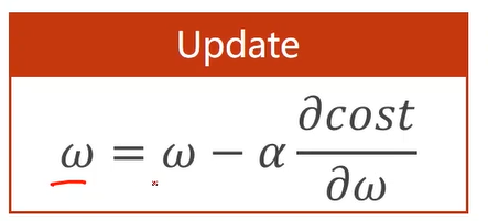
Algorithm explanation: when the partial derivative of the loss function to W is positive, it indicates that it is in the rising stage, that is, the value of the loss function should increase, and to find the minimum value of the loss function, w should be reduced; When the partial derivative of the loss function to W is negative, it indicates that it is currently in the decline stage, and the value of the loss function will decrease. In order to find the minimum value of the loss function, it is necessary to continue to increase W. among α It is the learning rate and controls the learning step, which is generally small.
If the loss function is non convex, it will be easy to be trapped in the local optimal position and can not find the global optimal position. As shown in the figure below:

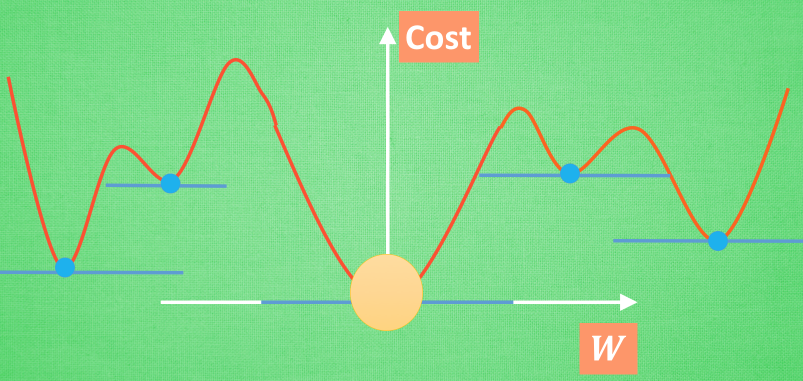
However, in the actual deep learning network, it is found that there are few local optima, so it will not be considered for the time being.
There is also a special case called saddle point, whose mathematical meaning is: the gradient (first derivative) value of the objective function at this point is 0, but one direction starting from the modified point is the maximum point of the function, and the other direction is the minimum point of the function. As shown in the following figure:

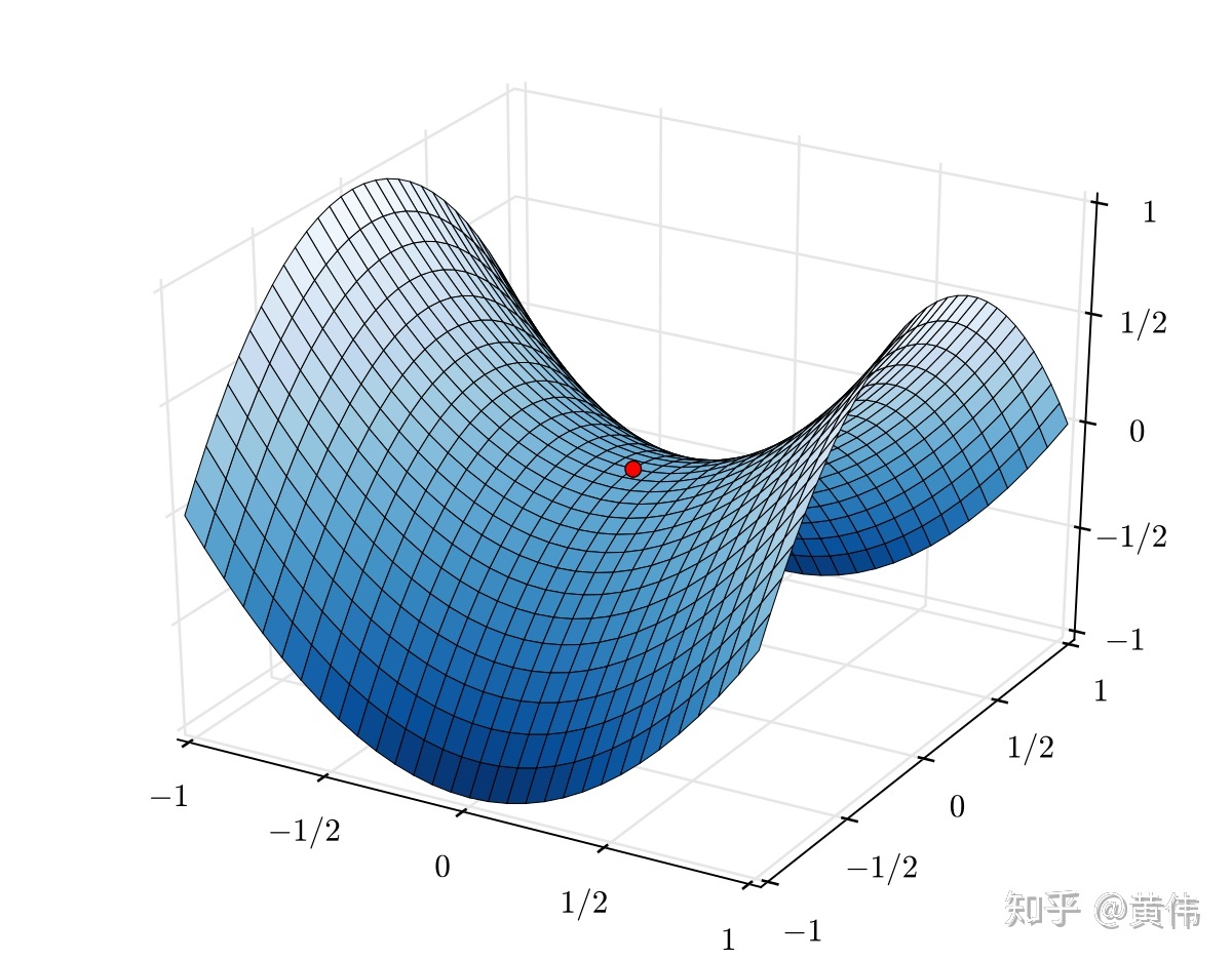
Saddle points can be solved by random gradient descent, which will be introduced in detail later.
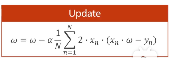
By substituting the previously used loss function into the updated formula w for simplification, we can get:

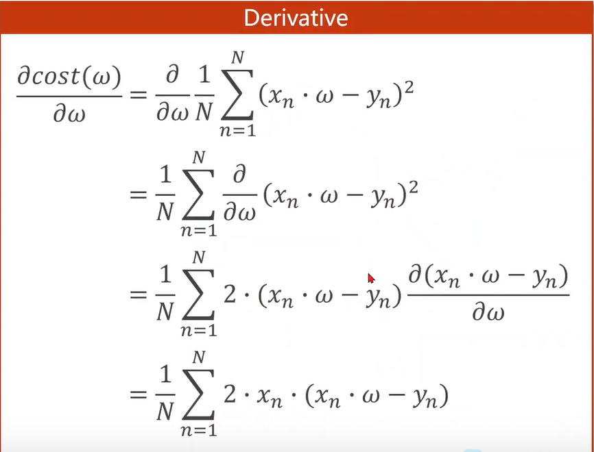
Therefore, the final gradient update formula is:

In practical application, stochastic gradient descent (SGD) will be used instead of gradient descent. The specific implementation process is as follows:

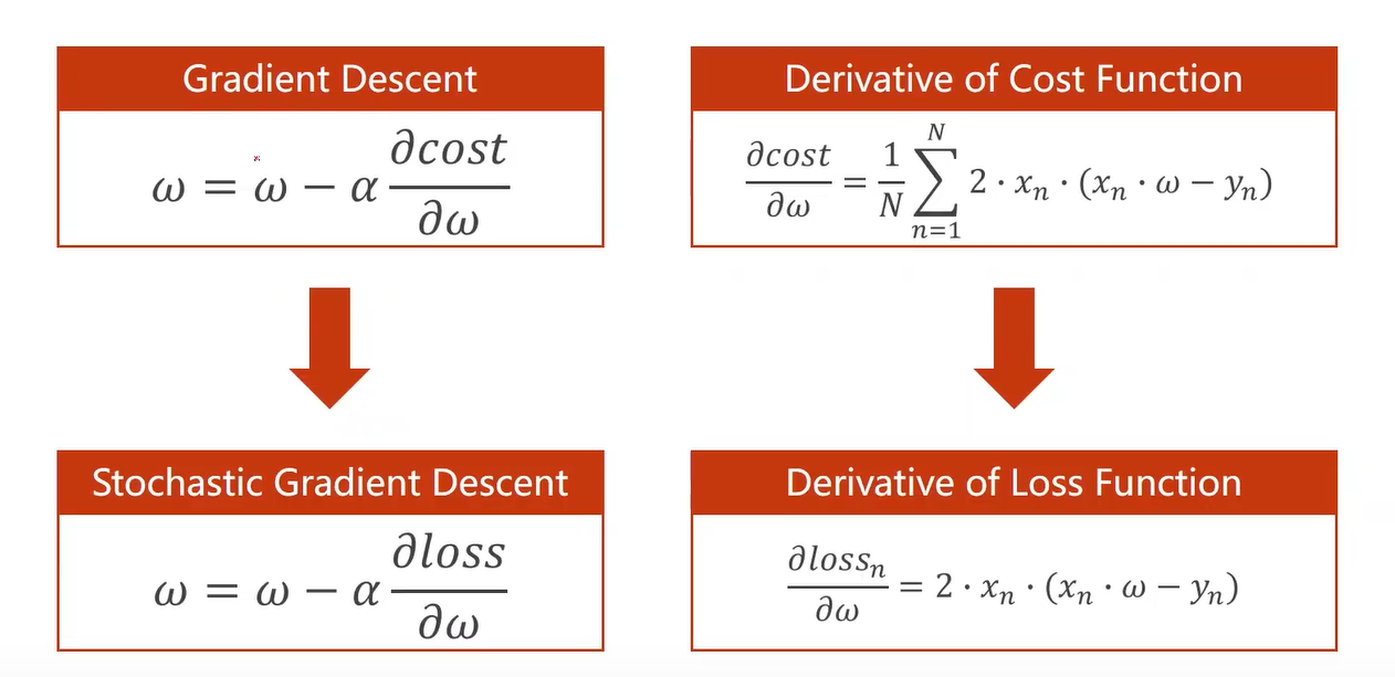
Different from gradient descent, the loss function cost() of all samples is replaced by the loss function loss() of a single random sample. The purpose of this is to reduce the influence of saddle point, which has been proved to be very effective in neural network.
However, it should also be noted that random gradient descent cannot process data in parallel like gradient descent, that is, gradient descent can ensure low time complexity but low performance, while random gradient descent can ensure prediction performance but high time complexity. Therefore, in deep learning, choose a compromise between the two and use Batch. (follow up)

code implementation

Weight update using gradient descent method:

# Import the library needed for drawing
import matplotlib.pyplot as plt

# Prepare data
x_data = [1.0, 2.0, 3.0]
y_data = [2.0, 4.0, 6.0]

# Initialize weight
w = 1.0

# Store the weight and corresponding loss value
cost_val_list = []
epoch_list = []

# Forward function
def forward(x):
    return x * w

# loss function 
def cost(xs, ys):
    cost = 0
    for x, y in zip(xs, ys):
        y_pred = forward(x)
        cost += (y_pred - y) ** 2
    return cost / len(xs)

# gradient descent 
def gradient(xs, ys):
    grad = 0
    for x, y in zip(xs, ys):
        grad += 2 * x * (x * w - y)
    return grad / len(xs)

print('Predict (before training)', 4, forward(4))
# Iterate
for epoch in range(100):
    cost_val = cost(x_data, y_data)
    grad_val = gradient(x_data, y_data)
    w -= 0.01 * grad_val
    print('Epoch', epoch, 'w=', w, 'loss=', cost_val)

    cost_val_list.append(cost_val)
    epoch_list.append(epoch)
print('Predict (after training)', 4, forward(4))

plt.plot(epoch_list, cost_val_list)
plt.ylabel('loss')
plt.xlabel('epoch')
plt.show()

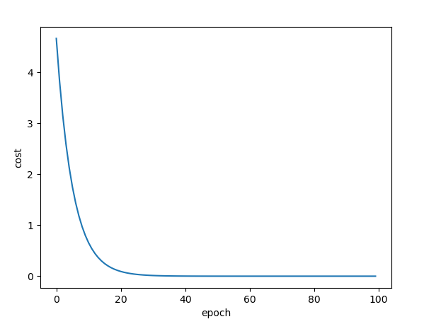
The correspondence between the number of iterations and the loss function is as follows:

Update weights using random gradient descent:

# Import the library needed for drawing
import matplotlib.pyplot as plt

# Prepare data
x_data = [1.0, 2.0, 3.0]
y_data = [2.0, 4.0, 6.0]

# Initialize weight
w = 1.0

# Store the weight and corresponding loss value
loss_val_list = []
epoch_list = []

# Forward function
def forward(x):
    return x * w

# loss function 
def loss(x, y):
    y_pred = forward(x)
    return (y_pred - y) ** 2

# gradient descent 
def gradient(x, y):
    return 2 * x * (x * w - y)

print('Predict (before training)', 4, forward(4))
# Iterate
for epoch in range(100):
    for x, y in zip(x_data, y_data):
        grad = gradient(x, y)
        w = w - 0.01 * grad
        print("\tgrad", x, y, grad)
        l = loss(x, y)
    print('Epoch', epoch, 'w=', w, 'loss=', l)
    loss_val_list.append(l)
    epoch_list.append(epoch)
print('Predict (after training)', 4, forward(4))

plt.plot(epoch_list, loss_val_list)
plt.ylabel('loss')
plt.xlabel('epoch')
plt.show()

The relationship between the corresponding loss function and the number of iterations is as follows:

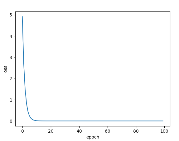
It can be seen from the figure that the random gradient descent algorithm drops faster than the gradient descent algorithm in the early stage.