pytorch learning
import torch
import numpy as np
a=torch.rand(4,3,28,28) #torch.rand(batch_size, channel, row, column)
a[0].shape #batch_ shape with size = 0:
torch.Size([3, 28, 28])
a[0,0].shape #batch_ shape with size = 0 and channel 0:
torch.Size([28, 28])
a[0,0,2,4] #batch_size=0, pixels in Row 2 and column 4 on the 0th channel
tensor(0.8694)
1. Slice
1.1 continuous sampling
[:] #all
[: n] # from 0 to n
[n:] # from n to end
[start:end] # start index: end index
a[:2].shape # ":" can be understood as →, that is, from the first picture to the second picture
torch.Size([2, 3, 28, 28])
a[:2,:1,:,:].shape #If no value is given,: indicates all
torch.Size([2, 1, 28, 28])
a[:2,1:,:,:].shape
torch.Size([2, 2, 28, 28])
a[:2,-1:,:,:].shape #Forward index [0,1,2], reverse index [- 3, - 2, - 1]
torch.Size([2, 1, 28, 28])
1.2 interlaced sampling
[start 🔚 Sampling step [step]
a[:,:,0:28:2,0:28:2].shape
torch.Size([4, 3, 14, 14])
a[:,:,::2,::2].shape
torch.Size([4, 3, 14, 14])
1.3 sampling by specific index
a.index_select(0,torch.tensor([0,2])).shape #For the 0-dimensional operation, sample the 0-th picture and the 2-th picture. Other dimensions remain unchanged
torch.Size([2, 3, 28, 28])
a.index_select(1,torch.tensor([1,2])).shape #For the first dimension operation, other dimensions remain unchanged
torch.Size([4, 2, 28, 28])
a.index_select(2,torch.arange(8)).shape #Operate on the line, and other dimensions remain unchanged
torch.Size([4, 3, 8, 28])
a.index_select(3,torch.arange(12)).shape #Operate on the column, and other dimensions remain unchanged
torch.Size([4, 3, 28, 12])
"..." is only for convenience
a[...].shape #"..." represents any number of dimensions, that is, all dimensions= a[:,:,:,:]
torch.Size([4, 3, 28, 28])
a[0,...].shape #=a[0,:,:,:]
torch.Size([3, 28, 28])
a[:,0,...].shape #=a[:,0,:,:]
torch.Size([4, 28, 28])
a[...,:2].shape #=a[:,:,:,:2] when "..." appears, the index on the right should be understood as the rightmost
torch.Size([4, 3, 28, 2])
a[0,...,::2].shape
torch.Size([3, 28, 14])
2. Dimension transformation
2.1.masked_select()
x = torch.randn(3,4)
x
tensor([[ 0.6480, 1.5947, 0.6264, 0.6051],
[ 1.6784, 0.2768, -1.8780, -0.1133],
[-0.6442, 0.8570, 0.1677, 0.2378]])
mask = x.ge(0.5)#ge(0.5) means "> = 0.5"
mask
tensor([[ True, True, True, True],
[ True, False, False, False],
[False, True, False, False]])
torch.masked_select(x,mask) #Take out the data of "> = 0.5"
tensor([0.6480, 1.5947, 0.6264, 0.6051, 1.6784, 0.8570])
torch.masked_select(x,mask).shape
torch.Size([6])
2.2 flatten index
src = torch.tensor([[4,3,5],[6,7,8]])
src
tensor([[4, 3, 5],
[6, 7, 8]])
torch.take(src,torch.tensor([0,2,5])) #After flattening the src
tensor([4, 5, 8])
2.3 view / reshape
a = torch.rand(4,1,28,28)
a.shape
torch.Size([4, 1, 28, 28])
a.view(4,28*28) #(4,1*28*28)
tensor([[0.6799, 0.1414, 0.2763, ..., 0.1316, 0.1727, 0.5590],
[0.4192, 0.5028, 0.3343, ..., 0.0582, 0.3610, 0.0597],
[0.7654, 0.6181, 0.8086, ..., 0.7929, 0.1571, 0.3276],
[0.5736, 0.3868, 0.4300, ..., 0.5922, 0.5513, 0.7693]])
a.view(4,28*28).shape
torch.Size([4, 784])
a.view(4*1*28,28).shape #Only care about column data, merge channels and rows together
torch.Size([112, 28])
a.view(4*1,28,28).shape #Only care about features_ Map, regardless of which channel it comes from. The data itself remains unchanged and becomes an understanding of the data
torch.Size([4, 28, 28])
b = a.view(4,784)
b#If you only look at b, you can't see the original storage method of data, that is, the four dimension information in a doesn't appear
tensor([[0.6799, 0.1414, 0.2763, ..., 0.1316, 0.1727, 0.5590],
[0.4192, 0.5028, 0.3343, ..., 0.0582, 0.3610, 0.0597],
[0.7654, 0.6181, 0.8086, ..., 0.7929, 0.1571, 0.3276],
[0.5736, 0.3868, 0.4300, ..., 0.5922, 0.5513, 0.7693]])
b.view(4,28,28,1).shape #Although this operation does not report an error, it destroys the information of the original data (4,1,28,28)
#The storage / dimensional order of data is very important. Only when the original data dimension information is obtained can b be restored to a
torch.Size([4, 28, 28, 1])
2.4 squeeze extrusion / unsqueeze deployment
a.shape
torch.Size([4, 1, 28, 28])
a.unsqueeze(0).shape #An additional dimension is inserted before the 0 index, which can be understood as the group
torch.Size([1, 4, 1, 28, 28])
a.unsqueeze(-1).shape #Insert an additional dimension at the end, which can be understood as the attribute of the pixel
torch.Size([4, 1, 28, 28, 1])
a.unsqueeze(4).shape #ditto. The parameter can be (- 5 ~ 0 ~ 4)
torch.Size([4, 1, 28, 28, 1])
a.unsqueeze(-4).shape
torch.Size([4, 1, 1, 28, 28])
a.unsqueeze(-5).shape
torch.Size([1, 4, 1, 28, 28])
a.unsqueeze(5).shape #Dimension allowed range exceeded
IndexError Traceback (most recent call last)
in
---->1 a.unsqueeze (5). Shape # exceeds the allowed range of dimensions
IndexError: Dimension out of range (expected to be in range of [-5, 4], but got 5)
a = torch.tensor([1.2,2.3])
a
tensor([1.2000, 2.3000])
a.shape
torch.Size([2])
a.unsqueeze(-1)
tensor([[1.2000],
[2.3000]])
a.unsqueeze(-1).shape
torch.Size([2, 1])
a.unsqueeze(0)
tensor([[1.2000, 2.3000]])
a.unsqueeze(0).shape
torch.Size([1, 2])
b = torch.rand(32)
b.shape
torch.Size([32])
f = torch.rand(4,32,14,14)
#bias is equivalent to adding an offset to all pixels on each channel
b = b.unsqueeze(1).unsqueeze(2).unsqueeze(0)
b.shape
torch.Size([1, 32, 1, 1])
After the above steps, b is changed from one dimension of torch.Size([32]) to four dimensions of torch.Size([1, 32, 1, 1])
b.squeeze().shape #Remove all of dimension=1
torch.Size([32])
b.squeeze(0).shape #Squeeze out dimension 0
torch.Size([32, 1, 1])
b.squeeze(-1).shape #Squeeze out the last dimension
torch.Size([1, 32, 1])
b.squeeze(1).shape #Squeeze out the first dimension
torch.Size([1, 32, 1, 1])
b.squeeze(-4).shape #Squeeze out - 4D
torch.Size([32, 1, 1])
3. Extension: the following two effects are the same
3.1 expand:broadcasting # only changes the understanding mode and does not add data
a = torch.rand(4,32,14,14)
b = b.unsqueeze(1).unsqueeze(2).unsqueeze(0)
b.shape
torch.Size([1, 1, 1, 1, 32, 1, 1])
b = torch.rand(1,32,1,1)
b.expand(4,32,14,14).shape   #Only if the original dimension is 1, it can be changed. The number that was not 1 should be copied
torch.Size([4, 32, 14, 14])
b.expand(-1,32,-1,-1).shape #-1 means the dimension remains unchanged
torch.Size([1, 32, 1, 1])
b.expand(-1,32,-1,-4).shape #-4 is a bug, and the generated result is meaningless
torch.Size([1, 32, 1, -4])
3.2 repeat:memory copied # add data
b.shape
torch.Size([1, 32, 1, 1])
b.repeat(4,32,1,1).shape #4 means 4 times for 0-dimensional copy, and 32 means 32 times for 1-dimensional copy. The repeat parameter indicates the number of repetitions.
torch.Size([4, 1024, 1, 1])
b.repeat(4,1,1,1).shape
torch.Size([4, 32, 1, 1])
b.repeat(4,1,32,32).shape
torch.Size([4, 32, 32, 32])
Transpose of matrix. t
a = torch.randn(3,4)
a.shape
torch.Size([3, 4])
a.t()
a.t().shape
torch.Size([4, 3])
Transfer implements pairwise exchange
a = torch.rand(4,3,32,32)
a1 = a.transpose(1,3).contiguous().view(4,3*32*32).view(4,3,32,32)
#This way of writing will cause data pollution. It is wrong. The last view should be (4,32,32,3), and then use transfer to change it back
#Correct writing: keep track of dimension information, remember dimension information when view ing, and expand by dimension without confusion
a2 = a.transpose(1,3).contiguous().view(4,3*32*32).view(4,32,32,3).transpose(1,3)
#Transfer contains two dimensions to be exchanged [b,c,h,w] → [b,w,h,c]
#The dimension order of the data must be consistent with the storage order. Use. Continuous to turn the data into continuous
#.view(4,3*32*32)  [b,w*h*c]
#.view(4,3,32,32)  [b,w,h,c]
#.transpose(1,3)   [b,c,g,w]
a1.shape,a2.shape
(torch.Size([4, 3, 32, 32]), torch.Size([4, 3, 32, 32]))
torch.all(torch.eq(a,a1))
tensor(False)
torch.all(torch.eq(a,a2))
tensor(True)
permute
a = torch.rand(4,3,28,28)
a.transpose(1,3).shape
torch.Size([4, 28, 28, 3])
b = torch.rand(4,3,28,32)             #b c h w
b.transpose(1,3).shape                #b w h c
torch.Size([4, 32, 28, 3])
b.transpose(1,3).transpose(1,2).shape #b h w c
torch.Size([4, 28, 32, 3])
#Through the above steps, we can change [b,c,h,w] into [b,h,w,c]
#You can complete the transformation directly with the index through permute
b.permute(0,2,3,1).shape #b h w c
torch.Size([4, 28, 32, 3])
#[b,h,w,c] is the format for storing pictures in numpy. It needs to be converted to this format before exporting numpy
broadcast: expand the dimension. copy data is not required during expansion
1. If there is no dimension in front, you need to insert a new dimension in front
2. Expand the newly added dimension to the same size. Example: A, B. B has no content. Insert a new dimension for B and expand B into the same dimension as a
3. After convolution neural network, feature maps are generated: [4,32,14,14]
4,Bias:32,1,1=>1,32,1,1=>4,32,14,14
why broadcasting?
for actual demanding:
·regulation:[class,student,score],add bias for every students: +5score
·because [4,32,8]can only add with [4,32,8],
·on the contrary,we hope [4,32,8]can add with [5.0](0dimension tensor)
key:Match from last dim
situation 1:
·if current dim=1,expand to same
    eg.A[4,32,8](four classes,32 students,8 lessons),now we want the score of each lesson be added 5.
    B[1] => B[1,1,1] => B[4,32,8]
A[4,32,14,14]
B[1,32,1,1] => [4,32,14,14]
situation 2:
·if either has no dim,insert one dim and expand to same
    now we just want the score of English be added 5
    B[1,1,8] => [4,32,8]   (through[0,0,5,0,0,0,0,0])
A[4,32,14,14]
B[14,14] => [1,1,14,14] =>[4,32,14,14]
situation 3:
·NOT broadcasting-able
A[4,32,14,14]
B[2,32,14,14]#dim 0 has distinct dim,NOT size 1,so cannot insert and expand to same
4.merge or split
4.1 cat is extended from the original dimension
a = torch.rand(4,32,8)
b = torch.rand(5,32,8)
torch.cat([a,b],dim=0).shape #dim=0 means merging in the 0 dimension. When merging, ensure that the A and B dimensions are the same, and the values of other dimensions are the same
torch.Size([9, 32, 8])
4.2 stack will create a new dimension
a1 = torch.rand(32,8)
b1 = torch.rand(32,8)
c = torch.stack([a1,b1],dim=0)  #Insert a new dimension before
c.shape
torch.Size([2, 32, 8])
torch.stack([a,b],dim=0).shape #The shape s of A1 and B1 are required to be identical
RuntimeError Traceback (most recent call last)
in
---->1 torch.stack ([a, b], dim = 0). shape # requires that the shapes of A1 and B1 are identical
RuntimeError: stack expects each tensor to be equal size, but got [4, 32, 8] at entry 0 and [5, 32, 8] at entry 1
4.3 split split by length len
c.shape
torch.Size([2, 32, 8])
aa,bb = c.split([1,1],dim=0) #Split the 0 dimension, [1,1] means "the length of the first block is 1, and the length of the second block is 1"
aa.shape,bb.shape
(torch.Size([1, 32, 8]), torch.Size([1, 32, 8]))
aa,bb = c.split(1,dim=0)
aa.shape,bb.shape
(torch.Size([1, 32, 8]), torch.Size([1, 32, 8]))
aa,bb = c.split(2,dim=0) #The total length is only 2, but if you want to split the length into 2, you can't split it
ValueError Traceback (most recent call last)
in
---->1 AA, BB = C. split (2, dim = 0) # length is only 2 in total, but it cannot be split if the length is split into 2
ValueError: not enough values to unpack (expected 2, got 1)
4.4 chunk s are split by quantity
c.shape
m,n = c.chunk(2,dim=0)#Split into 2 pieces
m.shape,n.shape
c.shape
5. Basic operation
5.1 add / minus / multiply / divid
a = torch.rand(3,4)
a
b = torch.rand(4)
b
a+b
torch.add(a,b)
torch.all(torch.eq(a-b,torch.sub(a,b)))
torch.all(torch.eq(a*b,torch.mul(a,b)))
torch.all(torch.eq(a/b,torch.div(a,b)))
#Note that the mathematical operator is equivalent to the English name. It is recommended to use the operator directly
5.2 matmul
(1)2d tensor matmul
#torch.mm is only applicable to 2d and is not recommended
#Torch.match is recommended. It can also be used directly@
a = torch.tensor([[3.,3.],[3.,3.]])
a
b = torch.ones(2,2)
b
torch.mm(a,b)
torch.matmul(a,b)
a@b
#Realize dimension reduction (4784) = > (4512)
a = torch.rand(4,784)
x = torch.rand(4,784)
w = torch.rand(512,784)  #channel-out,channel-in
(x@w.t()).shape          #. t() is only applicable to 2d tensor. If it is high-dimensional, use transfer
#Neural network can be understood as tensor, multiplication and addition of matrices
(2)>2d tensor matmul
a = torch.rand(4,3,28,64)
b = torch.rand(4,3,64,32)
a.shape,b.shape,torch.matmul(a,b).shape#The first two dimensions remain unchanged and the second two dimensions operate
b1 = torch.rand(4,1,64,32)
a.shape,b.shape,torch.matmul(a,b1).shape#broadcast and matrix multiplication are used
b2 = torch.rand(4,64,32)
torch.matmul(a,b2)
5.3 power matrix power
a = torch.full([2,2],3.)#Create a matrix with [2,2] shape of all 3
a.pow(2)    #Learn to use pow
a**2
aa = a**2
aa.sqrt() #square root
aa.rsqrt() #Reciprocal of square root
aa**(0.5) #Either square or square can be written like this
tensor([[[0.3398, 0.9368, 0.4789, 0.9124, 0.6989, 0.3476, 0.5464, 0.8225],
[0.6950, 0.3233, 0.8133, 0.8307, 0.9493, 0.7528, 0.7099, 0.3549],
[0.9476, 0.4018, 0.5350, 0.4714, 0.2160, 0.7102, 0.8838, 0.9494],
[0.8027, 0.9576, 0.7581, 0.9324, 0.9776, 0.7598, 0.6035, 0.6960],
[0.8669, 0.9793, 0.3580, 0.8107, 0.7291, 0.7721, 0.6947, 0.9367],
[0.9766, 0.3777, 0.4006, 0.9466, 0.7487, 0.9789, 0.9271, 0.7690],
[0.1329, 0.9046, 0.7036, 0.3389, 0.9362, 0.6187, 0.3904, 0.8272],
[0.7000, 0.8479, 0.9273, 0.7959, 0.3503, 0.4138, 0.8511, 0.7003],
[0.6475, 0.6537, 0.4819, 0.4237, 0.4267, 0.3168, 0.9740, 0.3920],
[0.4832, 0.6160, 0.8322, 0.6348, 0.1435, 0.6557, 0.9311, 0.5860],
[0.6276, 0.8570, 0.9184, 0.8391, 0.6393, 0.4581, 0.9451, 0.4369],
[0.7666, 0.7174, 0.9480, 0.9748, 0.6960, 0.9299, 0.8889, 0.1886],
[0.7654, 0.5772, 0.4515, 0.8861, 0.3661, 0.4661, 0.2333, 0.7668],
[0.5873, 0.6093, 0.9528, 0.1773, 0.7145, 0.6223, 0.2573, 0.6029],
[0.6388, 0.9341, 0.9153, 0.6012, 0.6718, 0.7056, 0.2280, 0.6289],
[0.6477, 0.7973, 0.9231, 0.6404, 0.5791, 0.6749, 0.8733, 0.7136],
[0.8370, 0.2390, 0.2808, 0.9373, 0.9406, 0.2357, 0.6042, 0.4712],
[0.4983, 0.6453, 0.8371, 0.8353, 0.6088, 0.7799, 0.5297, 0.3448],
[0.9584, 0.8916, 0.8728, 0.7693, 0.6398, 0.7883, 0.1654, 0.6025],
[0.6611, 0.1903, 0.9439, 0.7829, 0.9064, 0.7874, 0.5384, 0.5753],
[0.9957, 0.4825, 0.5329, 0.7879, 0.8094, 0.8641, 0.7971, 0.7981],
[0.9564, 0.6858, 0.8706, 0.7443, 0.9070, 0.6545, 0.6979, 0.9505],
[0.1372, 0.0457, 0.9959, 0.1995, 0.9982, 0.5210, 0.6383, 0.9822],
[0.8265, 0.6194, 0.8625, 0.9786, 0.9352, 0.1755, 0.5430, 0.6145],
[0.3293, 0.5944, 0.4495, 0.8490, 0.3312, 0.8978, 0.4665, 0.6412],
[0.9291, 0.6356, 0.9027, 0.8648, 0.3429, 0.8181, 0.5362, 0.8759],
[0.8120, 0.3447, 0.7006, 0.7554, 0.2462, 0.2694, 0.7855, 0.7590],
[0.9253, 0.5977, 0.7083, 0.8144, 0.9617, 0.7077, 0.6159, 0.9634],
[0.6062, 0.7896, 0.9842, 0.4307, 0.8408, 0.5411, 0.3181, 0.6006],
[0.8072, 0.7346, 0.6431, 0.0922, 0.5432, 0.7285, 0.2538, 0.4684],
[0.9054, 0.9919, 0.9948, 0.9246, 0.8321, 0.1768, 0.8794, 0.2131],
[0.8103, 0.9626, 0.8980, 0.6205, 0.5940, 0.6741, 0.5050, 0.9740]]])
5.4 Exp log
a = torch.exp(torch.ones(2,2))  #Based on e
a
tensor([[2.7183, 2.7183],
[2.7183, 2.7183]])
torch.log(a) #Write a few words based on who you are
tensor([[1., 1.],
        [1., 1.]])
5.5 approximate solution
.floor().ceil()
.round()
.trunc().frac()
a = torch.tensor(3.14)
a
tensor(3.1400)
a.floor(),a.ceil(),a.trunc(),a.frac()#floor goes down, ceil goes up, trunc is clipped to integer part and frac is clipped to decimal part
(tensor(3.), tensor(4.), tensor(3.), tensor(0.1400))
a = torch.tensor(3.499)
a.round()  #rounding
tensor(3.)
a = torch.tensor(3.5)
a.round()
tensor(4.)
5.6 clip clipping
gradient clipping
(min)
(min,max)
eg.for w in []
clamp(w.grad,10)
grad = torch.rand(2,3)*15
grad
tensor([[14.1900, 14.6534, 6.0197],
[ 7.3536, 5.4166, 11.4699]])
grad.max()
tensor(14.6534)
grad.median()
tensor(7.3536)
grad.clamp(10) #(min), change the unity less than 10 to 10
tensor([[14.1900, 14.6534, 10.0000],
[10.0000, 10.0000, 11.4699]])
grad
tensor([[14.1900, 14.6534, 6.0197],
[ 7.3536, 5.4166, 11.4699]])
grad.clamp(0,10) #(min,max)
tensor([[10.0000, 10.0000, 6.0197],
[ 7.3536, 5.4166, 10.0000]])
6. Attribute statistics
6.1 norm
norm-p
a = torch.full([8],1.)
a,a.dtype
(tensor([1., 1., 1., 1., 1., 1., 1., 1.]), torch.float32)
b = a.view(2,4)
b,b.dtype
(tensor([[1., 1., 1., 1.],
[1., 1., 1., 1.]]),
torch.float32)
c = a.view(2,2,2)
c,c.dtype
Output:
(tensor([[[1., 1.],
          [1., 1.]],

         [[1., 1.],
          [1., 1.]]]),
 torch.float32)
a.norm(1),b.norm(1),c.norm(1) #Expected floating point, not integer. 1 norm is the sum of absolute values
(tensor(8.), tensor(8.), tensor(8.))
a.norm(2),b.norm(2),c.norm(2) #The 2 norm is the square sum of the absolute values of all elements and the open root sign
(tensor(2.8284), tensor(2.8284), tensor(2.8284))
b.norm(1,dim=1) #1 norm of the first dimensional element
tensor([4., 4.])
b.norm(2,dim=1)#2 norm of the first dimensional element
tensor([2., 2.])
c.norm(1,dim=0)#1 norm of dimension 0 element
tensor([[2., 2.],
[2., 2.]])
c.norm(2,dim=0)#2 norm of element in the 0th dimension
tensor([[1.4142, 1.4142],
[1.4142, 1.4142]])
6.2 min,max,mean,sum,prod
a = torch.arange(8).view(2,4).float()
a
tensor([[0., 1., 2., 3.],
[4., 5., 6., 7.]])
a.min(),a.max(),a.mean(),a.sum(),a.prod() #Minimum, maximum, median, sum, multiply
(tensor(0.), tensor(7.), tensor(3.5000), tensor(28.), tensor(0.))
a.argmax(),a.argmin() #The index of the maximum value and the index of the minimum value. First flatten a and then give the index.
(tensor(7), tensor(0))
a.argmax(dim=0),a.argmin(dim=0)#Index of the row where the maximum / minimum value of the column is located
(tensor([1, 1, 1, 1]), tensor([0, 0, 0, 0]))
a.argmax(dim=1),a.argmin(dim=1)#The column index where the row maximum / minimum value is located
(tensor([3, 3]), tensor([0, 0]))
6.3 dim,keepdim
a.max(dim=1)
torch.return_types.max(
values=tensor([3., 7.]),
indices=tensor([3, 3]))
a.max(dim=1,keepdim=True)
torch.return_types.max(
values=tensor([[3.],
[7.]]),
indices=tensor([[3],
[3]]))
a.argmax(dim=1,keepdim=True)
tensor([[3],
[3]])
6.4 top-k or k-th
. topk maximum k
largest
kthvalue
a
tensor([[0., 1., 2., 3.],
[4., 5., 6., 7.]])
a.topk(3,dim=1) #The largest three numbers in the first dimension from large to small and their corresponding indexes
torch.return_types.topk(
values=tensor([[3., 2., 1.],
[7., 6., 5.]]),
indices=tensor([[3, 2, 1],
[3, 2, 1]]))
a.topk(3,dim=1,largest=False) #The value of the smallest three numbers in the first dimension from small to large and its corresponding index
torch.return_types.topk(
values=tensor([[0., 1., 2.],
[4., 5., 6.]]),
indices=tensor([[0, 1, 2],
[0, 1, 2]]))
a.kthvalue(4,dim=1) #The fourth smallest value in the first dimension, that is, the largest value
torch.return_types.kthvalue(
values=tensor([3., 7.]),
indices=tensor([3, 3]))
a.kthvalue(3) #The third smallest value is the second largest value
torch.return_types.kthvalue(
values=tensor([2., 6.]),
indices=tensor([2, 2]))
a.kthvalue(2,dim=1) #The second smallest value in the first dimension, that is, the third largest value
torch.return_types.kthvalue(
values=tensor([1., 5.]),
indices=tensor([1, 1]))
6.5 compare
torch.eq(a,b)
torch.eaqul(a,b)
a>0,a.dtype
(tensor([[False, True, True, True],
[ True, True, True, True]]),
torch.float32)
torch.gt(a,0) #gt is great, the same as above, indicating > 0
tensor([[False, True, True, True],
[ True, True, True, True]])
a != 0
tensor([[False, True, True, True],
[ True, True, True, True]])
b = torch.ones(2,3)
c = torch.randn(2,3)
b,c
(tensor([[1., 1., 1.],
[1., 1., 1.]]),
tensor([[-0.2182, -0.7458, -0.4226],
[-0.0562, -1.0081, 0.9595]]))
torch.eq(b,c)
tensor([[False, False, False],
[False, False, False]])
torch.equal(b,b)
True
7. High order operation
where Select source according to conditions,It can replace inconvenient loop logic control
    torch.where(condition,source x,source y)→tensor
    return a tensor of elements selected from either x or y,depending on condition:
    if condition,out_i = x_i,
      otherwise,out_i = y_i
gather Look up table
    torch.gather(input,dim,index,out=None)→tensor
    gather values along an axis specified by dim.
    for a 3-D tensor the output is specified by out[i][j][k]=input[i][j][index[i][j][k]]#if dim == 2
cond = torch.tensor([[0.6769,0.7271],[0.8884,0.4163]])
cond
tensor([[0.6769, 0.7271],
[0.8884, 0.4163]])
a = torch.full([2,2],0.)
a
tensor([[0., 0.],
[0., 0.]])
b = torch.full([2,2],1.)
b
tensor([[1., 1.],
[1., 1.]])
torch.where(cond>0.5,a,b)
tensor([[0., 0.],
[0., 1.]])
#retrieve global label
prob = torch.randn(4,10)
prob
tensor([[ 2.5846, 0.1205, 0.9951, -0.3636, 0.3576, 1.6804, -0.4364, -0.7844,
0.4014, 0.1721],
[ 3.4028, -0.1766, -0.7051, 1.3496, -0.8652, -1.1937, -0.0648, -1.0526,
-0.8368, -0.2342],
[-1.9581, 1.1129, 1.2058, -1.0913, 1.5528, 0.6695, 1.0291, 1.4307,
-1.2577, -0.7917],
[-0.2095, 0.6609, -0.7099, 0.6236, -1.5831, 0.6597, 1.2883, -1.1838,
-0.4961, -0.6793]])
idx = prob.topk(dim=1,k=3)
idx
torch.return_types.topk(
values=tensor([[ 2.5846, 1.6804, 0.9951],
[ 3.4028, 1.3496, -0.0648],
[ 1.5528, 1.4307, 1.2058],
[ 1.2883, 0.6609, 0.6597]]),
indices=tensor([[0, 5, 2],
[0, 3, 6],
[4, 7, 2],
[6, 1, 5]]))
idx = idx[1]
idx
tensor([[0, 5, 2],
[0, 3, 6],
[4, 7, 2],
[6, 1, 5]])
label = torch.arange(10)+100
label
tensor([100, 101, 102, 103, 104, 105, 106, 107, 108, 109])
torch.gather(label.expand(4,10),dim=1,index=idx.long())#Input, dimension, table
#50 and 6 correspond to 105100106 respectively
tensor([[100, 105, 102],
[100, 103, 106],
[104, 107, 102],
[106, 101, 105]])
8. Gradient
Derivative
Partial derivative
gradient # treats all partial differential equations as vectors
Convex functions are like bowls
Saddle point: take the minimum value of one dimension and the maximum value of the other dimension at one point
Influencing factors:
initialization initial state (initial position)
learning rate lr learning rate (can be adjusted to 0.001 first)
Escape minimum: add momentum (inertia)
Gradient ▽ = (partial differential of y to w, partial differential of y to b)
8.1 activation function
According to the frog experiment and the biological mechanism of biological neurons, it is found that:
The output of neural network is not a simple summation of each input, but has a threshold response mechanism.
Only values that meet the activation function conditions have output results.
There are only six activation functions available in machine learning: identity function, step function, sign, sigmoid, tanh, ReLU and softmax.
softmax and identity functions hardly appear on the hidden layer
sign and tanh hardly appear on the output layer
ReLU and sigmoid are widely used in hidden layer and output layer
Activation function (represented by h(z) if it is on the middle layer; If it is on the output layer, it is represented by g(z))
.
h(z): the activation function generally refers to the activation function on the hidden layer. The change of the activation function of the hidden layer will affect the output result. The activation functions on the same layer should be consistent to facilitate debugging (different settings can also be set)
g(z): the activation function on the output layer has no effect on the output result
(1) In order to solve the case that the step function is non differentiable, scientists proposed a continuous activation function: sigmoid:
f(x) = 1/(1+e^(-x))
·Differentiable, derivative to x = f(x)-f ²( x)=f(x)(1-f(x)), the derivative is the largest at point 0
·Value range (0,1)
·Disadvantages: when x becomes larger and larger, the derivative gradually approaches 0, and the derivative = f(x), the function cannot be updated for a long time, that is, gradient dispersion (gradient disappears)
·In practice, the relationship between variables is usually not a straight line, but a curve. In order to make the statistical model better fit the curve, statisticians introduce the link function on both sides of the linear regression equation to make various changes to the linear regression equation. The changed equation is called "generalized linear regression". Logarithmic function regression with logarithms on both sides of such as equation; At the same time, take exponential S-shaped function regression, etc. In this process, statisticians noticed the changes brought by sigmoid function:
·sigmoid can convert continuity variables into typed variables (for example, set the threshold to 0.5 when σ> 1 at 0.5, σ< (0 at 0.5)
·Take the result as a probability( σ/( 1- σ)) The z: ln of linear regression can be obtained( σ/( 1- σ))= Xw. Because of this property, the algorithm of adding sigmoid on both sides of the equal sign is called "logarithmic probability regression", which is logistic regression in English. Logistic regression is the most well-known algorithm in generalized linear regression. It is an algorithm called "regression" (the independent variable is linear). In fact, it is always used for classification[ σ Is the probability of the event, 1- σ Is the probability that the event will not happen, σ/( 1- σ) Is the relative probability that the sample is predicted to be 1. When the sample corresponds to σ The closer it is to 1 or 0, the more certain the prediction result of logistic regression on this sample is, and the higher the possibility that the sample is classified correctly; If σ Very close to the threshold indicates that the logistic regression is not very sure about the category of this sample.]
z = torch.linspace(-100,100,10)
z
tensor([-100.0000, -77.7778, -55.5556, -33.3333, -11.1111, 11.1111,
33.3333, 55.5556, 77.7778, 100.0000])
torch.sigmoid(z)#Change the value to (0,1)
tensor([0.0000e+00, 1.6655e-34, 7.4564e-25, 3.3382e-15, 1.4945e-05, 9.9999e-01,
1.0000e+00, 1.0000e+00, 1.0000e+00, 1.0000e+00])
(2) tanh English pronunciation / tai chi/
·=2*sigmoid(2x)-1
·Mostly used in RNN
·Value range (- 1,1)
·Center point (0,0), the derivative is the largest when the independent variable is 0
a = torch.linspace(-1,1,10)
a
tensor([-1.0000, -0.7778, -0.5556, -0.3333, -0.1111, 0.1111, 0.3333, 0.5556,
0.7778, 1.0000])
torch.tanh(a)#Value range (- 1,1)
tensor([-0.7616, -0.6514, -0.5047, -0.3215, -0.1107, 0.1107, 0.3215, 0.5047,
0.6514, 0.7616])
(3) ReLU(Rectified Linear Unit) is recommended to be used preferentially. It is a favorite in the field of neural networks. English pronunciation: / Rel you/
0, Z < 0 does not respond, and the derivative function is 0
z. Z > 0 response, derivative function is 1, no amplification and reduction, no gradient dispersion and gradient explosion
·Can be used to clear negative elements
·The derivative function is a step function
a
tensor([-1.0000, -0.7778, -0.5556, -0.3333, -0.1111, 0.1111, 0.3333, 0.5556,
0.7778, 1.0000])
torch.relu(a)
tensor([0.0000, 0.0000, 0.0000, 0.0000, 0.0000, 0.1111, 0.3333, 0.5556, 0.7778,
1.0000])
(4)Leaky ReLU
X < 0, y = ax (a is very small, generally 0.02)
x>0 , y = x
#The use method is very simple. Replace the original ReLU with leaky ReLU
self.model = nn.Sequential(
    nn.Linear(784,200),
    nn.LeakyReLU(inplace = True),
    nn.Linear(200,200),
    nn.LeakyReLU(inplace = True),
    nn.Linear(200,10),
    nn.LeakyReLU(inplace = True),
)
File "< ipython-input-150-8cfd5b39a69f>", line 4
nn.LeakyReLU(inplace = True),
^
SyntaxError: invalid character in identifier
(5) SELU: solve the problem of ReLU discontinuity at 0
(6) softplus: smooth the ReLU at 0
(7) Sign sign function (opposite sign on both sides of point 0), also known as step function 1, z > 0; 0,z=0; - 1, Z < 0 # rarely used
X = torch.tensor([[1,0,0],[1,1,0],[1,0,1],[1,1,1]],dtype=torch.float32)
andgate = torch.tensor([[0],[0],[0],[1]],dtype=torch.float32) #andgate = x1&x2
w = torch.tensor([-0.2,0.15,0.15],dtype=torch.float32)

def LinearRwithsign(X,w):
    zhat = torch.mv(X,w)
    andhat = torch.tensor([int(x) for x in zhat >= 0],dtype=torch.float32)
    return zhat,andhat

zhat,andhat = LinearRwithsign(X,w)
zhat,andhat
(tensor([-0.2000, -0.0500, -0.0500, 0.1000]), tensor([0., 0., 0., 1.]))
9.tipical loss
Basic optimization thought
The goal of model training is to make the output of neural network as close as possible to the real value.
Model training:
1) Define the basic model and make it clear that the goal is to solve the weight vector w
2) Define the loss function / objective function (a function to evaluate the difference between the real value and the predicted value, with the weight vector as the independent variable)
·Complex mathematical tools are required to solve the loss function:
·Lagrange transformation is a common mathematical method to transform loss function L(w) into convex function
·The method of solving w corresponding to the minimum value of L(w) on convex function is the optimization algorithm represented by gradient descent
For recurrent neural networks, the most common loss function is SSE=
3) Define optimization algorithm
4) Aiming at minimizing the loss function, the weight is solved
Loss function:
(1) MSE [mean square error]: used for regression
    ·MSELoss = (1/m)∑(zi-zihat)² = (L2_norm)² = (1/m)*∑(y Actual value-yhat Output value of the model)²
    ·
(2)SSE[sum of the Squared Errors]: SSE = ∑(zi-zihat)²
from torch.nn import MSELoss
yhat = torch.randn(size=(50,),dtype=torch.float32)
y = torch.randn(size=(50,),dtype=torch.float32)
#Class must be instantiated before use. criterion/loss is used for instantiation
criterion = MSELoss()#If you want to know whether a function has parameters, put the cursor in parentheses and press shift+Tab
loss = criterion(yhat,y)#Loss = criterion (real value, predicted value)
loss#Value of mean square error MSE
tensor(1.9280)
criterion = MSELoss(reduction = "sum")
#Mselos (reduction = "mean") indicates MSE (default)
#Mselos (reduction = "sum") indicates SSE
loss = criterion(yhat,y)#Loss = criterion (real value, predicted value)
loss
tensor(96.4017)
(3) Cross Entropy Loss, also known as logarithmic loss: used to classify entropy to represent "uncertainty"
    Cross entropy H(p,q) = -∑p(x)logq(x).
        ·When q More and more close to p When, H Getting closer to 0;
        ·When p=q,cross entropy value = entropy value

    ·binary: Second classification
        Maximum likelihood estimation solution: if you want something to happen, you should increase the probability of it, and you only need to find the weight to maximize its probability of occurrence w. Find the corresponding weight
                    w,The basic method of maximum likelihood estimation is to maximize the occurrence probability of target events.
            Steps:
            ①Construct likelihood function P(w),Used to evaluate the probability of target events. The function is designed to maximize the probability when the target event occurs
            ②The log likelihood function is formed by taking the logarithm of the overall likelihood function lnP(w)
            ③Weighting on log likelihood function w Find the derivative and make the derivative 0 to solve the weight

         P(yihat|xi,w) = P1^yi * P0^(1-yi),A hypothetical function mathematically called logistic regression. yi Represents the true label of the sample. At this time, the effect of the model is the best.
         Take both sides at the same time ln,To change a continuous multiplication into a continuous addition: lnP = ∑(yi*ln(σi) + (1-yi)*ln(1-σi))#σ i is the output of the activation function
         This is the binary cross entropy loss function.

         seek Loss We want to find the minimum, not the maximum. So add before“-"number:
         L(w)i = -∑(yi*ln(σi) + (1-yi)*ln(1-σi))   #σ i is the output of the activation function
         As long as the minimum value is obtained, the model can have the best fitting effect on the training data. The specific solution needs to use the optimization algorithm.

    ·multi-class: Multi classification
        Deep learning is basically: multi classification cross entropy loss
        Multi category labels no longer obey 0-1 Distribution.σfinger softmax Output of function
        Cross entropy function: L(w) = -∑yi_(k=j)ln(σi). Binary classification cross entropy function can be regarded as a special form of multi classification cross entropy function.

        When solving, the logarithmic operation is actually carried out after determining the likelihood function, but from the calculation results, the logarithmic operation is only effective softmax Result of functionσIt works.
        Therefore, in practice, the ln(softmax(z))A separate function is defined: logsoftmax,pytorch Can be passed directly through nn.logsoftmax Class calls this function
        At the same time, the processes other than logarithm, such as multiplying by label, adding and taking negative, are packaged, which is called negative log likelihood function( Negitive Log Likelihood function), stay pytorch of use nn.NLLLoss To make the call

    ·+softmax: And softmax Use with activation function
        ·softmax The tensor is scaled and each value is (0),1),And all the values add up=1
        ·Convert values into probabilities[2.0,1.0,0.1]→[0.7,0.2,0.1],Put the original large value larger, and compress the original small value into a more dense space. It turns out that 2 is two of 1
            Times, after change, 0.7 Is 0.2 Of 3.5 Times.
    ·leave it to logistic regression part
 Why not use for classification problems MSE?
    sigmoid+MSE: The gradient will disappear
    Cross entropy converges faster
    Note: if the effect of cross entropy is not good, it can be used MSE
#Loss = -(y*ln(sigma) + (1-y)*ln(1-sigma))
#y - true label
#Prediction probability of sigma binary classification - sigmoid(z)
#Z = XW, X is the characteristic tensor and w is the weight
#X,w
#m sample size
m = 3*pow(10,3)  #Scientific notation 3000
torch.random.manual_seed(420)
X = torch.rand((m,4),dtype=torch.float32)
w = torch.rand((4,1),dtype=torch.float32)
y = torch.randint(low=0,high=2,size=(m,1),dtype=torch.float32)#[0,2), so the value is 0,1. There are several labels for several samples
zhat = torch.mm(X,w)#metrix*metrix
sigma = torch.sigmoid(zhat)
sigma.shape
torch.Size([3000, 1])
loss = -(1/m)*sum(y*torch.log(sigma) + (1-y)*torch.log(1-sigma))  #(total loss)/m
loss
tensor([0.7962])
m = 3*pow(10,6)
torch.random.manual_seed(420)
X = torch.rand((m,4),dtype=torch.float32)#X.shape:[3000000,4]
w = torch.rand((4,1),dtype=torch.float32)
y = torch.randint(low=0,high=2,size=(m,1),dtype=torch.float32)#[0,2), so the value is 0,1. There are several labels for several samples
zhat = torch.mm(X,w)#metrix*metrix
sigma = torch.sigmoid(zhat)
import time#Observe two methods: sum / torch.sum operation time
start1 = time.time()#Capture current time in seconds
loss1 = -(1/m)*    sum  (y*torch.log(sigma) + (1-y)*torch.log(1-sigma))
now1 = time.time()#Capture current time in seconds
print(now1 - start1)
18.511772871017456
start2 = time.time()#Capture current time in seconds
loss2 = -(1/m)*torch.sum(y*torch.log(sigma) + (1-y)*torch.log(1-sigma))#As long as it is not a simple number addition and subtraction, you must use the function in torch: torch
now2 = time.time()#Capture current time in seconds
print(now2 - start2)
0.03202319145202637
"""
Because cross entropy loss is too common, it is pytorch There are special classes for calculation. Here are two nn Classes in modules:
class BCEWithLogitsLoss
    Built in sigmoid Function and cross entropy function, which will automatically calculate the input value sigmoid Value. Therefore, input is required zhat And real labels, and the order cannot be changed, zhat Must be before.

class BCELoss
    Only the cross entropy function, No sigmoid Layer. Therefore, input is required sigma And real labels, and the order cannot be changed

Both classes require the data type (must be floating point) and structure of the predicted value and the real label( shape)Must be the same, otherwise the operation will report an error.

"""
import torch.nn as nn
criterion1 = nn.BCELoss()#Instantiate bceloss (reduce = "mean" to get the average value / "sum" to get the addition result / "none" to get the matrix)
loss1 = criterion1(sigma,y)

criterion2 = nn.BCEWithLogitsLoss()#instantiation
loss2 = criterion2(zhat,y)  #Different from BCELoss input. The accuracy is higher than BCELoss.

loss1,loss2#You can see that the results are the same
(tensor(0.8685), tensor(0.8685))
"""
Deep learning is basically: multi classification cross entropy loss
LogSoftmax + Negtive Log Likelihood function
"""
import torch
import torch.nn as nn
m = 3*pow(10,3)
torch.random.manual_seed(420)
X = torch.rand((m,4),dtype=torch.float32)#X.shape:[3000000,4]
w = torch.rand((4,3),dtype=torch.float32)
y = torch.randint(low=0,high=3,size=(m,),dtype=torch.float32)#[0,3), so the value is 0,1. There are several labels for several samples
zhat = torch.mm(X,w)#metrix*metrix
#logsoftmax - log + softmax, input: zhat
#MLLLoss()
logsm = nn.LogSoftmax(dim=1)#instantiation
logsigma = logsm(zhat)
logsigma
tensor([[-1.1139, -0.8802, -1.3585],
[-1.0558, -0.8982, -1.4075],
[-1.0920, -1.0626, -1.1430],
...,
[-1.0519, -0.9180, -1.3805],
[-1.0945, -1.1219, -1.0798],
[-1.0276, -0.8891, -1.4649]])
criterion = nn.NLLLoss()#Calculate loss
criterion(logsigma,y.long())#y needs to be an integer, not a floating point. Because the cross entropy loss needs to convert the label to one hot, floating-point numbers are not accepted as the input of the label
tensor(1.1147)
"""
Easier way: call directly CrossEntropyLoss
    criterion = nn.CrossEntropyLoss()
    criterion(zhat,y.long())#Just enter zhat
"""
criterion = nn.CrossEntropyLoss()
criterion(zhat,y.long())#Just enter zhat
tensor(1.1147)
Pay attention to showing the network structure and flexibility, and use classes that do not contain output layer activation functions:
Usually in the Model class__ init__ The number of middle layers is consistent with the number of corresponding activation functions in the forward function. If a class with built-in sigmoid/logsoftmax function is used to calculate the loss function,
The forward function will be defined with one less layer (output layer), and the network structure display is not simple and clear enough.
For complex networks, clear structure is more important.
At the same time, if the activation function is written separately, it becomes easy to modify the activation function. If it is mixed in the loss function, you have to change the code of the whole loss function when you want to modify the activation function, which is not conducive to maintenance.
Pay attention to stability and operation accuracy, and use the class containing the output layer activation function:
If the activation function of the output layer is not modified in a Model for a long time, considering the stable operation of the Model, the class with built-in activation function is used to calculate the loss function.
At the same time, the built-in activation function can help push up the accuracy of the operation.
'\ n pay attention to showing the network structure and flexibility. You should use classes that do not contain output layer activation functions: \ n usually in the Model class__ init__ The number of middle layers is consistent with the number of corresponding activation functions in the forward function. If the class with built-in sigmoid/logsoftmax function is used to calculate the loss function, \ the forward function will be defined with one less layer (output layer), and the network structure display is not simple and clear\ N for complex networks, clear structure is more important\ N at the same time, if the activation function is written separately, it becomes easy to modify the activation function. If it is mixed in the loss function, you have to change the code of the whole loss function when you want to modify the activation function, which is not conducive to maintenance\ N \ n pay attention to stability and operation accuracy, and use the class containing the activation function of the output layer: \ n if the activation function of the output layer is not modified in a Model for a long time, considering the stable operation of the Model, use the class with built-in activation function to calculate the loss function\ N at the same time, the built-in activation function can help push up the accuracy of the operation\ n\n’
How to use pytorch to automatically derive:
Method 1: torch.autograd.grad(loss,[w1,w2,...])
    [w1 grad,w2 grad...]
Method 2: loss.backward()
  Call method:
    w1.grad
    w2.grad
9.1 entropy: the sum of the amount of information. The greater the amount of information, the greater the entropy, the more certain the event, and the less the sense of surprise
a = torch.full([4],1/4.)
a
tensor([0.2500, 0.2500, 0.2500, 0.2500])
-(a*torch.log2(a)).sum()
tensor(2.)
a = torch.tensor([0.1,0.1,0.1,0.7])
-(a*torch.log2(a)).sum()
tensor(1.3568)
a = torch.tensor([0.001,0.001,0.001,0.999])
-(a*torch.log2(a)).sum()
tensor(0.0313)
#Data stability
from torch.nn import functional as F
x = torch.randn(1,784)
w = torch.randn(10,784)
logits = x@w.t()
pred = F.softmax(logits,dim=1)
pred_log = torch.log(pred)
F.cross_entropy(logits,torch.tensor([3]))  #cross_ The first parameter in tropy must be logits
tensor(16.1506)
F.nll_loss(pred_log,torch.tensor([3])) #cross_entropy = softmax + log + nll_loss
tensor(16.1506)
9.2 multi classification: put softmax before the output layer.
·In multi classification, the number of neurons is consistent with the number of labels. For example, if it is ten classification, there will be ten neurons on the output layer, which output ten different probabilities respectively. At this time, the prediction label of the sample is the label category corresponding to the largest probability of all output probabilities.
·softmax molecule is an exponential function of the regression results of a label category under multi classification
The denominator is the sum of the exponential functions of the regression results of all label categories under multi classification
The result of the softmax function represents the probability that the result of the sample is class k
For example, there are three categories: apple, pear and passion fruit. The probability that sample i is classified as passion fruit is: σ Passion fruit = e_z passion fruit / (E)_ Z Apple + e_z pear + e_z passion fruit)
Because the denominator and numerator of softmax have an exponential function with e as the bottom, it is very easy to have huge values in the calculation. If the number exceeds the limited data width required by the computer processing room, and the computer cannot calculate and express, this phenomenon is called "overflow".
from torch.nn import functional as F
x = torch.ones(1)
w = torch.full([1],2.)
mse = F.mse_loss(torch.ones(1),x*w) #(predict,label)
x,w,mse
(tensor([1.]), tensor([2.]), tensor(1.))
torch.autograd.grad(mse,[w]) #W is not set to require derivative information during initialization, so w does not need derivation by default
---------------------------------------------------------------------------

RuntimeError                              Traceback (most recent call last)

<ipython-input-161-e91b20e3e3cd> in <module>
----> 1 torch.autograd.grad(mse,[w]) #W is not set to require derivative information during initialization, so w does not need derivation by default


D:\anaconda\lib\site-packages\torch\autograd\__init__.py in grad(outputs, inputs, grad_outputs, retain_graph, create_graph, only_inputs, allow_unused)
    200         retain_graph = create_graph
    201
--> 202     return Variable._execution_engine.run_backward(
    203         outputs, grad_outputs_, retain_graph, create_graph,
    204         inputs, allow_unused)


RuntimeError: element 0 of tensors does not require grad and does not have a grad_fn
w.requires_grad_()#Must be a floating point number. Update the w information and tell pytorch that w needs derivation
tensor([2.], requires_grad=True)
torch.autograd.grad(mse,[w])#The reason for the error here is that w is a dynamic graph, that is, update step by step. The picture here is still the original one
---------------------------------------------------------------------------

RuntimeError                              Traceback (most recent call last)

<ipython-input-163-3cc9e23d25a7> in <module>
----> 1 torch.autograd.grad(mse,[w])#The reason for the error here is that w is a dynamic graph, that is, update step by step. The picture here is still the original one


D:\anaconda\lib\site-packages\torch\autograd\__init__.py in grad(outputs, inputs, grad_outputs, retain_graph, create_graph, only_inputs, allow_unused)
    200         retain_graph = create_graph
    201
--> 202     return Variable._execution_engine.run_backward(
    203         outputs, grad_outputs_, retain_graph, create_graph,
    204         inputs, allow_unused)


RuntimeError: element 0 of tensors does not require grad and does not have a grad_fn
mse = F.mse_loss(torch.ones(1),x*w)#to update
torch.autograd.grad(mse,[w])#Find the partial derivative of loss to w
(tensor([2.]),)
mse = F.mse_loss(torch.ones(1),x*w)#to update
mse.backward()#Another way to find partial derivatives. In the process of forward propagation, pytorch will record all paths. Therefore, it propagates from back to front on the last loss node
w.grad   #Cannot run multiple times
tensor([2.])
import torch
from torch.nn import functional as F
#softmax
a = torch.rand(3)
a.requires_grad_()
tensor([0.0983, 0.3098, 0.4726], requires_grad=True)
p = F.softmax(a,dim=0)#Operate on the feature dimension
p
tensor([0.2710, 0.3349, 0.3941], grad_fn=<SoftmaxBackward>)
p.backward() # requires_grad=True only applies once. It has been cleared in the second run and needs to be reset
---------------------------------------------------------------------------

RuntimeError                              Traceback (most recent call last)

<ipython-input-168-40f625a2e25d> in <module>
----> 1 p.backward() # requires_grad=True only applies once. It has been cleared in the second run and needs to be reset


D:\anaconda\lib\site-packages\torch\tensor.py in backward(self, gradient, retain_graph, create_graph)
    219                 retain_graph=retain_graph,
    220                 create_graph=create_graph)
--> 221         torch.autograd.backward(self, gradient, retain_graph, create_graph)
    222
    223     def register_hook(self, hook):


D:\anaconda\lib\site-packages\torch\autograd\__init__.py in backward(tensors, grad_tensors, retain_graph, create_graph, grad_variables)
    124
    125     grad_tensors_ = _tensor_or_tensors_to_tuple(grad_tensors, len(tensors))
--> 126     grad_tensors_ = _make_grads(tensors, grad_tensors_)
    127     if retain_graph is None:
    128         retain_graph = create_graph


D:\anaconda\lib\site-packages\torch\autograd\__init__.py in _make_grads(outputs, grads)
     48             if out.requires_grad:
     49                 if out.numel() != 1:
---> 50                     raise RuntimeError("grad can be implicitly created only for scalar outputs")
     51                 new_grads.append(torch.ones_like(out, memory_format=torch.preserve_format))
     52             else:


RuntimeError: grad can be implicitly created only for scalar outputs
p = F.softmax(a,dim=0)
torch.autograd.grad(p[1],[a],retain_graph=True)  #When i is equal to j, the gradient is positive and the rest is negative. i is 1, so in [0,1,2], only the value corresponding to index 1 is positive
(tensor([-0.0908, 0.2227, -0.1320]),)
torch.autograd.grad(p[2],[a])
(tensor([-0.1068, -0.1320, 0.2388]),)
(2) softmax overflow
z = torch.tensor([1010,100,999],dtype=torch.float32)
torch.exp(z)/torch.sum(torch.exp(z))#Data overflow occurred
tensor([nan, nan, nan])
torch.softmax(z,0)       #No overflow
#Softmax can only calculate data in a single dimension. Therefore, even if the input is one-dimensional, you need to specify the dimension index during softmax operation, otherwise an error will be reported
#From the output results, 1010 has the greatest probability. The input value is the largest and the output result is the largest.
#Therefore, if you do not need to know the specific output probability, you can directly see the output result from the input value without softmax
tensor([9.9998e-01, 0.0000e+00, 1.6701e-05])
z = torch.tensor([10,9,5],dtype=torch.float32)
torch.exp(z)/torch.sum(torch.exp(z))
tensor([0.7275, 0.2676, 0.0049])
torch.softmax(z,0)
tensor([0.7275, 0.2676, 0.0049])
torch.softmax(z,0).sum() #The sum of probabilities is 1
tensor(1.)
Note: dimension parameters of softmax(,)
s = torch.tensor([[[1,2,4,5],[3,4,4,5],[5,6,4,5]],[[5,6,4,5],[7,8,4,5],[9,10,4,5]]],dtype=torch.float32)
s,s.shape
#It means that a tensor has two two-dimensional tables, each table has three rows, and each row has four elements
(tensor([[[ 1.,  2.,  4.,  5.],
          [ 3.,  4.,  4.,  5.],
          [ 5.,  6.,  4.,  5.]],

         [[ 5.,  6.,  4.,  5.],
          [ 7.,  8.,  4.,  5.],
          [ 9., 10.,  4.,  5.]]]),
 torch.Size([2, 3, 4]))
s.shape[0],s.shape[1],s.shape[2]#Forward index
(2, 3, 4)
s.shape[-3],s.shape[-2],s.shape[-1]#Negative index
(2, 3, 4)
torch.softmax(s,dim=0)#The sum of the probabilities of each two-dimensional table is 1
tensor([[[0.0180, 0.0180, 0.5000, 0.5000],
         [0.0180, 0.0180, 0.5000, 0.5000],
         [0.0180, 0.0180, 0.5000, 0.5000]],

        [[0.9820, 0.9820, 0.5000, 0.5000],
         [0.9820, 0.9820, 0.5000, 0.5000],
         [0.9820, 0.9820, 0.5000, 0.5000]]])
torch.softmax(s,dim=1)#The sum of elements in each table and column is 1
tensor([[[0.0159, 0.0159, 0.3333, 0.3333],
         [0.1173, 0.1173, 0.3333, 0.3333],
         [0.8668, 0.8668, 0.3333, 0.3333]],

        [[0.0159, 0.0159, 0.3333, 0.3333],
         [0.1173, 0.1173, 0.3333, 0.3333],
         [0.8668, 0.8668, 0.3333, 0.3333]]])
torch.softmax(s,dim=2)#On each table, the sum of the elements on each row is 1
tensor([[[0.0128, 0.0347, 0.2562, 0.6964],
         [0.0723, 0.1966, 0.1966, 0.5344],
         [0.1966, 0.5344, 0.0723, 0.1966]],

        [[0.1966, 0.5344, 0.0723, 0.1966],
         [0.2562, 0.6964, 0.0128, 0.0347],
         [0.2671, 0.7262, 0.0018, 0.0049]]])
9.3 using cross_entropy for multi category combat
w1,b1 = torch.randn(200,784,requires_grad = True),torch.zeros(200,requires_grad = True) #torch.randn(ch-out,ch-in)
w2,b2 = torch.randn(200,200,requires_grad = True),torch.zeros(200,requires_grad = True)
w3,b3 = torch.randn(10,200,requires_grad = True),torch.zeros(10,requires_grad = True)  #Ten categories, so the output is 10

def forward(x):
    x = x@w1.t() + b1  #x point multiplied by weight 1 + offset 1
    x = F.relu(x)      #Activate function relu
    x = x@w2.t() + b2  #x point multiplied by weight 2 + offset 2
    x = F.relu(x)      #Activate function relu
    x = x@w3.t() + b3  #x point multiplied by weight 3 + offset 3
    x = F.relu(x)      #After activation, the relu function calls logits without softmax/sigmoid. This step can also be output directly without relu
    return x
import torch
from torch import nn
from torch import optim

epochs = 10
optimizer = optim.SGD([w1,b1,w1,b2,w3,b3],lr = 1e-3) #optimizer
criteon = nn.CrossEntropyLoss()

for epoch in range(epochs):
    for batch_idx,(data,target) in enumerate(train_loader):
        data = data.view(-1,28*28)

        logits = forward(data)  #Don't add softmax
        loss = criteon(logits,target)

        optimizer.zero_grad()
        loss.backward()
        optimizer.step()
9.4 principle and implementation of binary classification neural network
(1) tensor realizes forward propagation of binary classification neural network
import torch
X = torch.tensor([[1,0,0],[1,1,0],[1,0,1],[1,1,1]],dtype=torch.float32)
X#The first column represents constant neurons, the second column represents x1, and the second column represents x2
tensor([[1., 0., 0.],
[1., 1., 0.],
[1., 0., 1.],
[1., 1., 1.]])
andgate = torch.tensor([[0],[0],[0],[1]],dtype=torch.float32) #andgate = x1&x2
def LogisticR(X,w):#def LogisticR
    w = torch.tensor([-0.2,0.15,0.15],dtype=torch.float32)
    zhat = torch.mv(X,w)
    sigma = 1/(1 + torch.exp(-zhat))    #sigmoid For arguments sigma definition  #It can also be written as sigma = torch.sigmoid(zhat)
    andhat = torch.tensor([int(x) for x in sigma >= 0.5],dtype=torch.float32)  #The threshold is set artificially. The label greater than the threshold is 1 and the label less than the threshold is 0
    #In python, int(True)=1, int (flame) = 0. Put it directly into the list derivation and convert the Boolean value to 0 and 1
    return sigma,andhat
sigma,andhat = LogisticR(X,w)
sigma,andhat
(tensor([0.4502, 0.4875, 0.4875, 0.5250]), tensor([0., 0., 0., 1.]))
andgate #The result of andhat is the same as that of andgate. Remember: all that adds hat is the predicted value
tensor([0., 0., 0., 1.])
Drawing
(1)AND GATE
import matplotlib.pyplot as plt
import seaborn as sns
X = torch.tensor([[1,0,0],[1,1,0],[1,0,1],[1,1,1]],dtype=torch.float32)
#Set a canvas
plt.figure(figsize=(5,3))#Set canvas size
plt.scatter(X[:,1],X[:,2]#Take the column with X index 1 as X and the column with X index 2 as y
           ,c=andgate    #andgate has two values: 0 and 1. Color = category of real label
           ,cmap="rainbow"#Use the two colors with high contrast in the rainbow color
           )#Scatter plot
#Beautify pictures
plt.style.use('seaborn-whitegrid')#Set the style of the image
sns.set_style("white")
plt.title("AND GATE",fontsize=16)#Set image title
plt.xlim(-1,3)                   #Set abscissa dimension
plt.ylim(-1,3)                   #Set ordinate dimension
plt.grid(alpha=.4,axis="y")      #Displays the grid in the background
plt.gca().spines["top"].set_alpha(.0)#Let the upper axis be hidden
plt.gca().spines["right"].set_alpha(.0)#Make the right axis hidden
#Draw decision boundary
import numpy as np
x = np.arange(-1,3,0.5)#(- 1,3) regularly arranged data
plt.plot(x,(0.23-0.15*x)/0.15
        ,color="k",linestyle="--");
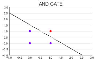
In a two-dimensional plane, any line can be represented as x1 = ax2 + b
 Change it, 0 = b - x1 + ax2
         0 = [1 - x1 + x2] * [b,-1,a].T
         0 = Xw
X Is the characteristic tensor, w Is the weight vector (column vector by default)
    When w,b When fixed, the straight line is fixed.
    When w,b When not fixed, a straight line is any straight line.

The point above the line is class 0( z <= 0),The point below the line is class 1( z > 0)#It can be realized by step function
 The line with classification function is called decision boundary
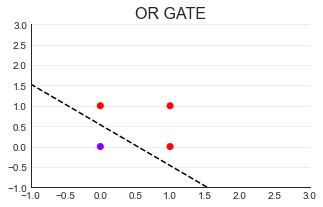
(2)OR GATE
import torch
X = torch.tensor([[1,0,0],[1,1,0],[1,0,1],[1,1,1]],dtype=torch.float32)
orgate = torch.tensor([0,1,1,1],dtype=torch.float32)
def OR(X):
    w = torch.torch.tensor([-0.08,0.15,0.15],dtype=torch.float32)
    zhat = torch.mv(X,w)
    yhat = torch.tensor([int(x) for x in zhat >= 0.5],dtype=torch.float32)
    return orgate
import matplotlib.pyplot as plt
import seaborn as sns
#Set a canvas
plt.figure(figsize=(5,3))#Set canvas size
plt.scatter(X[:,1],X[:,2]#Take the column with X index 1 as X and the column with X index 2 as y
           ,c=orgate    #andgate has two values: 0 and 1. Color = category of real label
           ,cmap="rainbow"#Use the two colors with high contrast in the rainbow color
           )#Scatter plot
#Beautify pictures
plt.style.use('seaborn-whitegrid')#Set the style of the image
sns.set_style("white")
plt.title("OR GATE",fontsize=16)#Set image title
plt.xlim(-1,3)                   #Set abscissa dimension
plt.ylim(-1,3)                   #Set ordinate dimension
plt.grid(alpha=.4,axis="y")      #Displays the grid in the background
plt.gca().spines["top"].set_alpha(.0)#Let the upper axis be hidden
plt.gca().spines["right"].set_alpha(.0)#Make the right axis hidden
#Draw decision boundary
import numpy as np
x = np.arange(-1,3,0.5)#(- 1,3) regularly arranged data
plt.plot(x,(0.08-0.15*x)/0.15
        ,color="k",linestyle="--");
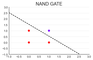
(3)NAND GATE
import torch
X = torch.tensor([[1,0,0],[1,1,0],[1,0,1],[1,1,1]],dtype=torch.float32)
nandgate = torch.tensor([1,1,1,0],dtype=torch.float32)
def NAND(X):
    w = torch.torch.tensor([0.23,-0.15,-0.15],dtype=torch.float32)
    zhat = torch.mv(X,w)
    yhat = torch.tensor([int(x) for x in zhat >= 0],dtype=torch.float32)
    return nandgate

import matplotlib.pyplot as plt
import seaborn as sns
#Set a canvas
plt.figure(figsize=(5,3))#Set canvas size
plt.scatter(X[:,1],X[:,2]#Take the column with X index 1 as X and the column with X index 2 as y
           ,c=nandgate    #andgate has two values: 0 and 1. Color = category of real label
           ,cmap="rainbow"#Use the two colors with high contrast in the rainbow color
           )#Scatter plot
#Beautify pictures
plt.style.use('seaborn-whitegrid')#Set the style of the image
sns.set_style("white")
plt.title("NAND GATE",fontsize=16)#Set image title
plt.xlim(-1,3)                   #Set abscissa dimension
plt.ylim(-1,3)                   #Set ordinate dimension
plt.grid(alpha=.4,axis="y")      #Displays the grid in the background
plt.gca().spines["top"].set_alpha(.0)#Let the upper axis be hidden
plt.gca().spines["right"].set_alpha(.0)#Make the right axis hidden
#Draw decision boundary
import numpy as np
x = np.arange(-1,3,0.5)#(- 1,3) regularly arranged data
plt.plot(x,(0.23-0.15*x)/0.15
        ,color="k",linestyle="--");
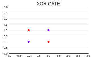
import torch
X = torch.tensor([[1,0,0],[1,1,0],[1,0,1],[1,1,1]],dtype=torch.float32)
xorgate = torch.tensor([0,1,1,0],dtype=torch.float32)

import matplotlib.pyplot as plt
import seaborn as sns
#Set a canvas
plt.figure(figsize=(5,3))#Set canvas size
plt.scatter(X[:,1],X[:,2]#Take the column with X index 1 as X and the column with X index 2 as y
           ,c=xorgate    #andgate has two values: 0 and 1. Color = category of real label
           ,cmap="rainbow"#Use the two colors with high contrast in the rainbow color
           )#Scatter plot
#Beautify pictures
plt.title("XOR GATE",fontsize=16)#Set image title
plt.xlim(-1,3)                   #Set abscissa dimension
plt.ylim(-1,3)                   #Set ordinate dimension
plt.grid(alpha=.4,axis="y")      #Displays the grid in the background
plt.gca().spines["top"].set_alpha(.0)#Let the upper axis be hidden
plt.gca().spines["right"].set_alpha(.0)#Make the right axis hidden
sigma_nand = NAND(X)#Return to nandgate
sigma_nand
tensor([1., 1., 1., 0.])
sigma_or = OR(X)#Return to orgate
sigma_or
tensor([0., 1., 1., 1.])
x0 = torch.tensor([1,1,1,1],dtype=torch.float32)
x0
tensor([1., 1., 1., 1.])
input_2 = torch.cat((x0.view(4,1),sigma_nand.view(4,1),sigma_or.view(4,1)),dim=1)#Merge tensor s, and the spliced contents shall be framed with () or []
input_2
#Specify the direction with dim, dim=0, and the three tensors are transversely spliced into tensors ([1,1,1,1,0,1,1,1,0,1,1.]);
#dim=1, the three tensors are arranged in columns
#Because x0,sigma_nand,sigma_or is a one-dimensional tensor without dim=1. Therefore, we need to change the three tensors into two-dimensional: use view to change into the specified appearance
tensor([[1., 1., 0.],
[1., 1., 1.],
[1., 1., 1.],
[1., 0., 1.]])
import torch
X = torch.tensor([[1,0,0],[1,1,0],[1,0,1],[1,1,1]],dtype=torch.float32)
andgate = torch.tensor([0,0,0,1],dtype=torch.float32)
def AND(X):
    w = torch.torch.tensor([-0.2,0.15,0.15],dtype=torch.float32)
    zhat = torch.mv(X,w)
    andhat = torch.tensor([int(x) for x in zhat >= 0],dtype=torch.float32)
    return andhat
AND(input_2)
tensor([0., 1., 1., 0.])
#All nonlinear problems must be realized by multilayer neural network
9.4 GPU acceleration
device = torch.device('cuda:0')
net = MLP().to(device)
optimizer = optim.SGD([net.parameters()],lr = learning_rate) #optimizer
criteon = nn.CrossEntropyLoss().to(device)

for epoch in range(epochs):
    for batch_idx,(data,target) in enumerate(train_loader):
        data = data.view(-1,28*28)
        data,target = data.to(device),target.cuda()   #. to(device) is equivalent to. CUDA (), except that. to(device) is the CPU and GPU cuda() can only specify GPU,
10. Chain rule
Forward propagation: calculate all variable values to the right before derivation
10.1 single layer sensor:
(1) Single layer (only one layer output) linear regression neural network: (characteristic input) input signal > artificial neuron > signal output (prediction result output)
The number of layers of neural network does not include "input layer"
Zhat (prediction result of Z) = wi * xi + b. Expressed as a matrix: zhat = XW (the column with 1 in X is specially used to multiply the weight)
Why z not y? In deep learning, y always represents the label. Because the output of deep learning is not a label, you don't need y. Generally, lower case letters in bold are used to represent column vectors, and upper case letters in bold are used to represent matrices or determinants. In machine learning, all one-dimensional vectors are column vectors by default.
The task of linear regression: fitting.
The essence of prediction function is the model to be built, and the core of prediction function is to find out the parameter vector w of the model
The vertical arrangement is called a layer. There is only one feature on a neuron. The number of neurons = the number of features + 1 (1 refers to the neuron corresponding to the deviation). The output layer has at least one neuron. The connecting lines are called axons,
x = torch.randn(1,10)                        #input
w = torch.randn(1,10,requires_grad = True)  #Weight, w dimension is 1
o = torch.sigmoid(x@w.t())                  #Activate function (input @ weight)
o.shape
torch.Size([1, 1])
loss = F.mse_loss(torch.ones(1,1),o)
loss.shape
torch.Size([])
loss.backward()
w.grad
tensor([[-0.1313, 0.0248, 0.0298, -0.0075, -0.0821, 0.0185, 0.0354, 0.0332,
-0.0105, 0.0642]])
Example: calculate the result of Z. z=b + w1x1 + w2x2
import torch
#For pytorch, in many cases, the two parameter types for operation are required to be the same
#It is recommended to define the data type when defining the tensor. Moreover, if an integer is not required, it is always set to float type and set to float32 (32 saves memory compared with 64). If an error is reported, adjust again.
X = torch.tensor([[1,0,0],[1,1,0],[1,0,1],[1,1,1]]
                 ,dtype = torch.float32)
#It can also be written as floating point:
#X = torch.tensor([[1,0,0],[1,1,0],[1,0,1],[1,1,1]])
#X.float()
w = torch.tensor([-0.2,0.15,0.15]) #(b,w1,w2)b at the front, the position of offset and weight can be changed according to the position of the column with matrix 1 (the column corresponding to the weight)
X,w
(tensor([[1., 0., 0.],
[1., 1., 0.],
[1., 0., 1.],
[1., 1., 1.]]),
tensor([-0.2000, 0.1500, 0.1500]))
def LinearR(X,w):   #Colon ":" don't forget that R means Regression
    zhat = torch.mv(X,w)#mv is a matrix * vector specific function MatrixVector
    return zhat
zhat = LinearR(X,w)   #Linear parameters must be of the same type
zhat#Estimate
tensor([-0.2000, -0.0500, -0.0500, 0.1000])
torch.Tensor([[1,0,0],[1,1,0],[1,0,1],[1,1,1]])#Tensor generates floating point numbers
tensor([[1., 0., 0.],
[1., 1., 0.],
[1., 0., 1.],
[1., 1., 1.]])
The difference between tensor and tensor:
torch.tensor will first judge the input data type, and then determine the data type in tensor according to it
torch.Tensor no matter what the input data is, it will output float32 without brain
z = torch.tensor([-0.2000, -0.0500, -0.0500,  0.1000])#True value
z.ndim  #dimension
1
zhat == z #The "inequality" here must not be the reason for the data type.
tensor([ True, False, False, False])
#SSE = SIGMA (real predicted) * 2)
zhat-z
tensor([0.0000e+00, 3.7253e-09, 3.7253e-09, 7.4506e-09])
SSE = sum((zhat - z)**2)
SSE#As can be seen from SSE, zhat and z are indeed unequal
tensor(8.3267e-17)
torch.set_printoptions(precision=30)#Print option: print 30 decimal places
zhat,z
#Reasons for Inequality:
#float32 has an accuracy problem because it only retains 32 bits
#When calculating torch.mv function, there will be very small internal problems
(tensor([[0.695239484310150146484375000000],
         [0.566381037235260009765625000000],
         [1.094140648841857910156250000000],
         [0.965282201766967773437500000000]], grad_fn=<AddmmBackward>),
 tensor([-0.200000002980232238769531250000, -0.050000000745058059692382812500,
         -0.050000000745058059692382812500,  0.100000001490116119384765625000]))
preds = torch.ones(300,68,64,64)
preds.shape
torch.Size([300, 68, 64, 64])
a = 300*68*64*64
a#How much data are there
83558400
preds = torch.ones(300,68,64,64) * 0.1
preds.sum() * 10   #It is found that * 0.1 and * 10 bring accuracy problems.
#Therefore, if the accuracy of the results is high, you need to set the float64 accuracy when creating. Note that float64 can only be reduced and can not eliminate the accuracy problem.
tensor(83558328.)
preds = torch.ones(300,68,64,64)
preds.sum()
tensor(83558400.)
torch.allclose(zhat,z)#. allclose() can help ignore small differences (you can set the threshold manually) to compare whether the two tensors are consistent
True
(2) torch.nn.Linear (representing the output layer, which is a subclass of nn.modal) realizes the forward propagation of single-layer recurrent neural network
There is no need to define w,b when using.
The input layer is determined by the characteristic matrix, so there is no need to define the input layer in the neural network, so when a network has several layers, it is not considered as the input layer.
The z generated by this method is only a random number similar to the characteristic matrix structure, and the neural network has not been told to predict the correct result
torch.set_printoptions(precision=4)#Adjust printing options: print 4 decimal places
X = torch.tensor([[0,0],[1,0],[0,1],[1,1]],dtype=torch.float32)
X#X does not need to set aside a special column of 1 for deviation
tensor([[0., 0.],
[1., 0.],
[0., 1.],
[1., 1.]])
#Instantiate nn.Linear. w,b will be generated automatically and randomly
output = torch.nn.Linear(2,1)
#Torch.nn.linear (the number of neurons in the upper layer that are transmitted to this layer, and the number of neurons in this layer that receive data transmitted from the upper layer)
#                 , bias = true by default).
#If bias is not required, write output = torch.nn.Linear(2,1, bias = False). At this time, output.bias returns nothing
zhat = output(X)
zhat
tensor([[ 0.1788],
[-0.0734],
[ 0.1401],
[-0.1121]], grad_fn=)
output.weight,output.bias#View automatically randomly generated w,b
(Parameter containing:
tensor([[-0.2522, -0.0387]], requires_grad=True),
Parameter containing:
tensor([0.1788], requires_grad=True))
#If you don't want W and B to be random, set the random number seed. Select one of many groups W and B of the system
torch.random.manual_seed(420)#Artificially set random number seeds.
#The numbers are set randomly. Each number corresponds to a mode. The computer is not very clear about which mode it corresponds. We just need to lock it. It is set to 420 here
output = torch.nn.Linear(2,1)
zhat = output(X)
zhat,zhat.shape#The z generated by this method is only a random number similar to the characteristic matrix structure, and the neural network has not been told to predict the correct result
(tensor([[0.6730],
[1.1048],
[0.2473],
[0.6792]], grad_fn=),
torch.Size([4, 1]))
(3) torch.functional realizes the forward propagation of single-layer binary neural network = > that is, logical regression
The only difference between logical regression and linear regression is that sigmoid function is set after the result of linear regression
As long as the output result of nn.Linear passes through the sigmoid function, the forward propagation of logical regression can be realized
#Classes are called out in nn.module, and functions are called out in nn.functional
import torch
from torch.nn import functional as F  #Abbreviate the function as F, so that you can call the function directly, such as F.sigmoid()
X = torch.tensor([[0,0],[1,0],[0,1],[1,1]],dtype=torch.float32)
torch.random.manual_seed(420)
dense = torch.nn.Linear(2,1)#Instantiate torch
zhat = dense(X) #dense means "close", which means that most of the neural networks in the upper layer are closely connected with this layer, which means the whole connection layer
sigma = F.sigmoid(zhat)
y = [int(x) for x in sigma >= 0.5]
y#Since W and B are randomly generated, y only needs to look at the format, and the content does not need to focus on whether it is the same as the result of andgate
[1, 1, 1, 1]
#sign
zhat,torch.sign(zhat) #z> 0 returns all 1
(tensor([[0.6730],
[1.1048],
[0.2473],
[0.6792]], grad_fn=),
tensor([[1.],
[1.],
[1.],
[1.]], grad_fn=))
#ReLU
F.relu(zhat)#>0 returns the original value, < 0 returns 0
tensor([[0.6730],
[1.1048],
[0.2473],
[0.6792]], grad_fn=)
#tanh
torch.tanh(zhat)#Zhat > 0, so all the returned results are located in (0,1)
tensor([[0.5869],
[0.8022],
[0.2424],
[0.5910]], grad_fn=)
10.2 multi layer perceptron:
x = torch.randn(1,10)
w = torch.randn(2,10,requires_grad = True)
o = torch.sigmoid(x@w.t())
o.shape
torch.Size([1, 2])
loss = F.mse_loss(torch.ones(1,2),o)
loss
tensor(0.5097, grad_fn=)
loss.backward()
w.grad
tensor([[ 0.0167, 0.0093, 0.0218, -0.0144, 0.0156, -0.0078, -0.0311, -0.0236, 0.0132, 0.0180],
[ 0.0020, 0.0011, 0.0026, -0.0017, 0.0019, -0.0009, -0.0037, -0.0028, 0.0016, 0.0022]])
w.grad.shape
torch.Size([2, 10])
Neural networks are black boxes
The process from left to right is the forward propagation process of neural network. The layer on the left is called "upper layer", and the layer on the right is called "lower layer". The input is layer 0, and the first hidden layer is called layer 1.
Neurons are numbered from top to bottom, 1,2.
The difference between different neurons is the activation function used after addition (represented by h(z) if it is on the middle layer; If it is on the output layer, it is represented by g(z). Z is the result of addition, σ Is the result of the activation function after the addition.
z and σ It is located on neurons, and w and b are located at the junction between layers.
The neural network is very complex. It is impossible to find out each W and B.
So deep learning doesn't pay much attention to interpretability, because we don't know how neural networks do it. It is very difficult to trace the input characteristics from the final results.
W of a single-layer neural network is a column vector, but in a multi-layer neural network, W is a matrix because there are multiple layers and multiple groups of W values.
Z shall be consistent with the order of feature labels. In order for Z to maintain the column vector, we need to write W before X, that is, the column row, n_featuresn_samples
It is the activation function on the hidden layer that makes the neural network have the ability to deal with linear and nonlinear problems. If the function is not activated, the output result is invalid
The affine transformation is still a linear transformation, which can not solve the nonlinear problem. It can be seen that "layer" itself is not the key to solve the nonlinear problem of neural network,
h(z) on the layer is. If h(z) is a linear function or does not exist, it is useless to add more layers.
You can try to put the above AND,OR,NAND Comment out the activation function of or replace it with another activation function and observe the output result.
Forward propagation of deep neural network from 0:
"""
Title: suppose there are 500 data and 20 features, and the label is divided into 3 categories.
Now we need to implement a three-layer neural network: the first layer has 13 neurons, the second layer has 8 neurons, and the third layer is the output layer.
The activation function of the first layer is relu,The activation function of the second layer is sigmoid.
The implementation code is as follows:
"""
import torch
import torch.nn as nn
from torch.nn import functional as F
#Determine data
torch.random.manual_seed(420)#Lock random number seed
x = torch.rand((500,20),dtype=torch.float32)
y = torch.randint(low=0,high=3,size=(500,1),dtype=torch.float32)#randint randomly generated integer (0,3]
#W will be generated automatically when nn.Linear is instantiated, so w does not need to be defined
#Inherit nn.Model class to complete forward propagation torch.nn - > nn.Model, nn.functional
class Model(nn.Module):#Enter the name of the parent class you want to inherit in parentheses
    def __init__(self,in_features=10,out_features=2):
        """
    Used to define class Model The class itself. nn.Module This class has thousands of lines of code, including init Function code accounts for the majority.
    The first parameter in parentheses is fixed self,Represents the class itself.
    in_features Represents the number of features input to the neural network (the number of neurons on the input layer), out_features Represents the characteristic number of the output of the neural network (the number of neurons on the output layer).
        """

        super(Model,self).__init__()
        """
    super Help inherit parent classes for more details.
    Name of sub module to inherit[lookup Model Parent module of nn.Model,hold nn.model Medium__init__Copy all to subclass__init__Yes.]
    without super In this line, the child class cannot inherit the parent class init Function, the following layers of neural network can not be defined.
        """
        self.Linear1 = nn.Linear(in_features,13,bias=True) #(number of upper neurons, number of lower neurons)
        self.Linear2 = nn.Linear(13,8,bias=True)
        self.output = nn.Linear(8,out_features,bias=True)

    def forward(self,x):#Neural network forward propagation
        #first floor
        z1 = self.Linear1(x)#Linear layer
        sigma1 = torch.relu(z1)#Output result of activation function
        #The second floor
        z2 = self.Linear2(sigma1)#Linear addition result
        sigma2 = torch.sigmoid(z2)#sigmoid results
        #Output layer
        z3 = self.output(sigma2)
        sigma3 = F.softmax(z3,dim=1)#Three neurons on the output layer, three output results. Calculate the first dimension of softmax and get the probability of three categories
        return sigma3
x.shape#x has 20 columns, so the number of neurons on the input layer should be 20
torch.Size([500, 20])
x.shape[1],y.unique()#Non duplicate labels in y
(20, tensor([0., 1., 2.]))
input_ = x.shape[1]
output_ = len(y.unique())
input_,output_
(20, 3)
#Instantiated neural network
torch.random.manual_seed(420)
net = Model(in_features=input_,out_features=output_)
net.forward(x).shape  #500 rows, 3 columns, 500 samples, 3 output categories
#The effect is equivalent to net(x). Because__ init__ There is only one function below, so when you enter net(x), it will be executed automatically__ init__ All functions defined below
torch.Size([500, 3])
net.Linear1.weight.shape#Matrix on the first linear layer.shape #x(500,20)
torch.Size([13, 20])
#W (13,20) * (20500) first transpose the characteristic matrix - > (13500)
net.Linear2.weight.shape
torch.Size([8, 13])
#w(8,13) * (13,500) -> (8,500)
net.output.weight.shape
torch.Size([3, 8])
#w(3,8) * (8,500) ->(3,500). When softmax is output, it is changed to (500,3)
net.Linear1.bias.shape#Enter the first hidden layer from the input layer. Because the first layer has 13 neurons, the bias.shape of the first layer is 3
torch.Size([13])
super function
#Create a parent class
class FooParent(object):
    def __init__(self):
        self.parent = 'PARENT!!'#attribute
        print('Running __init__,I am parent')
    def bar(self,message):
        self.bar = "This is bar"
        print("%s from Parent" % message)
FooParent()#The parent class instantiates the pair of instantaneously and runs its own__ init__
Running __init__,I am parent


<__main__.FooParent at 0x1f35c5da6a0>
FooParent().parent#The parent class runs its own__ init__ Properties defined in
Running __init__,I am parent


'PARENT!!'
#Create a subclass and make the subclass inherit the methods and properties of the parent class by calling the class name
class FooChild(FooParent):
    def __init__(self):
        print("Running __init__,I am child")
FooChild().bar("HAHAHA")#Check whether the subclass inherits the method
Running __init__,I am child
HAHAHA from Parent
FooChild().parent #The child class does not inherit from the parent class__ init__ The properties defined in only inherit__ init__ Functions other than
Running __init__,I am child


---------------------------------------------------------------------------

AttributeError                            Traceback (most recent call last)

<ipython-input-46-1aa4e3354ad7> in <module>
----> 1 FooChild().parent #The child class does not inherit from the parent class__ init__ Properties defined in


AttributeError: 'FooChild' object has no attribute 'parent'
#Create a subclass and use the super function
class FooChild(FooParent):
    def __init__(self):
        super(FooChild,self).__init__()#If you want a subclass to inherit from the parent class__ init__ For the attributes defined in, you need to use super()
        #The meaning of super is to find the parent class of FooChild and inherit it__ init__
        print("I am running __init__,I am child")
FooChild().parent#Call the parent attribute again to perform the init function of the child class and the function defined by the init function of the parent class
Running __init__,I am parent
I am running __init__,I am child


'PARENT!!'
#Inheritance of attributes
net.training#Is this class used for training now? If yes, return True; Otherwise, False is returned
True
#Method inheritance
#net.cuda()      #Transfer the whole network to GPU for
#net.cpu()       #Transfer the entire network to the CPU for
#net.apply()     #For all layers in the neural network, all objects in the init function perform the same operation
#net.Linear1.weight.data.fill_(0)#Fill all elements in the tensor with 0 at one time

def initial_0(m):#Let W and B all be 0
    print(m)
    if type(m) == nn.Linear:
        m.weight.data.fill_(0)
        print(m.weight)
net.apply(initial_0)
Linear(in_features=20, out_features=13, bias=True)
Parameter containing:
tensor([[0., 0., 0., 0., 0., 0., 0., 0., 0., 0., 0., 0., 0., 0., 0., 0., 0., 0., 0., 0.],
        [0., 0., 0., 0., 0., 0., 0., 0., 0., 0., 0., 0., 0., 0., 0., 0., 0., 0., 0., 0.],
        [0., 0., 0., 0., 0., 0., 0., 0., 0., 0., 0., 0., 0., 0., 0., 0., 0., 0., 0., 0.],
        [0., 0., 0., 0., 0., 0., 0., 0., 0., 0., 0., 0., 0., 0., 0., 0., 0., 0., 0., 0.],
        [0., 0., 0., 0., 0., 0., 0., 0., 0., 0., 0., 0., 0., 0., 0., 0., 0., 0., 0., 0.],
        [0., 0., 0., 0., 0., 0., 0., 0., 0., 0., 0., 0., 0., 0., 0., 0., 0., 0., 0., 0.],
        [0., 0., 0., 0., 0., 0., 0., 0., 0., 0., 0., 0., 0., 0., 0., 0., 0., 0., 0., 0.],
        [0., 0., 0., 0., 0., 0., 0., 0., 0., 0., 0., 0., 0., 0., 0., 0., 0., 0., 0., 0.],
        [0., 0., 0., 0., 0., 0., 0., 0., 0., 0., 0., 0., 0., 0., 0., 0., 0., 0., 0., 0.],
        [0., 0., 0., 0., 0., 0., 0., 0., 0., 0., 0., 0., 0., 0., 0., 0., 0., 0., 0., 0.],
        [0., 0., 0., 0., 0., 0., 0., 0., 0., 0., 0., 0., 0., 0., 0., 0., 0., 0., 0., 0.],
        [0., 0., 0., 0., 0., 0., 0., 0., 0., 0., 0., 0., 0., 0., 0., 0., 0., 0., 0., 0.],
        [0., 0., 0., 0., 0., 0., 0., 0., 0., 0., 0., 0., 0., 0., 0., 0., 0., 0., 0., 0.]],
       requires_grad=True)
Linear(in_features=13, out_features=8, bias=True)
Parameter containing:
tensor([[0., 0., 0., 0., 0., 0., 0., 0., 0., 0., 0., 0., 0.],
        [0., 0., 0., 0., 0., 0., 0., 0., 0., 0., 0., 0., 0.],
        [0., 0., 0., 0., 0., 0., 0., 0., 0., 0., 0., 0., 0.],
        [0., 0., 0., 0., 0., 0., 0., 0., 0., 0., 0., 0., 0.],
        [0., 0., 0., 0., 0., 0., 0., 0., 0., 0., 0., 0., 0.],
        [0., 0., 0., 0., 0., 0., 0., 0., 0., 0., 0., 0., 0.],
        [0., 0., 0., 0., 0., 0., 0., 0., 0., 0., 0., 0., 0.],
        [0., 0., 0., 0., 0., 0., 0., 0., 0., 0., 0., 0., 0.]],
       requires_grad=True)
Linear(in_features=8, out_features=3, bias=True)
Parameter containing:
tensor([[0., 0., 0., 0., 0., 0., 0., 0.],
        [0., 0., 0., 0., 0., 0., 0., 0.],
        [0., 0., 0., 0., 0., 0., 0., 0.]], requires_grad=True)
Model(
  (Linear1): Linear(in_features=20, out_features=13, bias=True)
  (Linear2): Linear(in_features=13, out_features=8, bias=True)
  (output): Linear(in_features=8, out_features=3, bias=True)
)


Model(
  (Linear1): Linear(in_features=20, out_features=13, bias=True)
  (Linear2): Linear(in_features=13, out_features=8, bias=True)
  (output): Linear(in_features=8, out_features=3, bias=True)
)
net.parameters()
<generator object Module.parameters at 0x000001F35C6174A0>
for param in net.parameters():
    print(param)#Print, observe the parameters iterator and find that it contains all weights and intercepts. Be sure to master parameters.
Parameter containing:
tensor([[0., 0., 0., 0., 0., 0., 0., 0., 0., 0., 0., 0., 0., 0., 0., 0., 0., 0., 0., 0.],
        [0., 0., 0., 0., 0., 0., 0., 0., 0., 0., 0., 0., 0., 0., 0., 0., 0., 0., 0., 0.],
        [0., 0., 0., 0., 0., 0., 0., 0., 0., 0., 0., 0., 0., 0., 0., 0., 0., 0., 0., 0.],
        [0., 0., 0., 0., 0., 0., 0., 0., 0., 0., 0., 0., 0., 0., 0., 0., 0., 0., 0., 0.],
        [0., 0., 0., 0., 0., 0., 0., 0., 0., 0., 0., 0., 0., 0., 0., 0., 0., 0., 0., 0.],
        [0., 0., 0., 0., 0., 0., 0., 0., 0., 0., 0., 0., 0., 0., 0., 0., 0., 0., 0., 0.],
        [0., 0., 0., 0., 0., 0., 0., 0., 0., 0., 0., 0., 0., 0., 0., 0., 0., 0., 0., 0.],
        [0., 0., 0., 0., 0., 0., 0., 0., 0., 0., 0., 0., 0., 0., 0., 0., 0., 0., 0., 0.],
        [0., 0., 0., 0., 0., 0., 0., 0., 0., 0., 0., 0., 0., 0., 0., 0., 0., 0., 0., 0.],
        [0., 0., 0., 0., 0., 0., 0., 0., 0., 0., 0., 0., 0., 0., 0., 0., 0., 0., 0., 0.],
        [0., 0., 0., 0., 0., 0., 0., 0., 0., 0., 0., 0., 0., 0., 0., 0., 0., 0., 0., 0.],
        [0., 0., 0., 0., 0., 0., 0., 0., 0., 0., 0., 0., 0., 0., 0., 0., 0., 0., 0., 0.],
        [0., 0., 0., 0., 0., 0., 0., 0., 0., 0., 0., 0., 0., 0., 0., 0., 0., 0., 0., 0.]],
       requires_grad=True)
Parameter containing:
tensor([ 1.3508e-01,  1.5439e-01, -1.9350e-01, -6.8777e-02,  1.3787e-01,
        -1.8474e-01,  1.2763e-01,  1.8031e-01,  9.5152e-02, -1.2660e-01,
         1.4317e-01, -1.4945e-01,  3.4258e-05], requires_grad=True)
Parameter containing:
tensor([[0., 0., 0., 0., 0., 0., 0., 0., 0., 0., 0., 0., 0.],
        [0., 0., 0., 0., 0., 0., 0., 0., 0., 0., 0., 0., 0.],
        [0., 0., 0., 0., 0., 0., 0., 0., 0., 0., 0., 0., 0.],
        [0., 0., 0., 0., 0., 0., 0., 0., 0., 0., 0., 0., 0.],
        [0., 0., 0., 0., 0., 0., 0., 0., 0., 0., 0., 0., 0.],
        [0., 0., 0., 0., 0., 0., 0., 0., 0., 0., 0., 0., 0.],
        [0., 0., 0., 0., 0., 0., 0., 0., 0., 0., 0., 0., 0.],
        [0., 0., 0., 0., 0., 0., 0., 0., 0., 0., 0., 0., 0.]],
       requires_grad=True)
Parameter containing:
tensor([ 0.0900, -0.0597,  0.0268, -0.0173,  0.0065,  0.0228, -0.1408,  0.1188],
       requires_grad=True)
Parameter containing:
tensor([[0., 0., 0., 0., 0., 0., 0., 0.],
        [0., 0., 0., 0., 0., 0., 0., 0.],
        [0., 0., 0., 0., 0., 0., 0., 0.]], requires_grad=True)
Parameter containing:
tensor([-0.0156, -0.0730, -0.2637], requires_grad=True)
10.3 chain rule: solve complex gradients through product
ay/ax = (ay/au) * (au/ax)
x = torch.tensor(1.)
w1 = torch.tensor(2.,requires_grad = True)
b1 = torch.tensor(1.)
w2  = torch.tensor(2.,requires_grad = True)
b2 = torch.tensor(1.)
y1 = x*w1+b1
y2 = y1*w2+b2
dy2_dy1 = torch.autograd.grad(y2,[y1],retain_graph = True)[0]
dy1_dw1 = torch.autograd.grad(y1,[w1],retain_graph = True)[0]
dy2_dw1 = torch.autograd.grad(y2,[w1],retain_graph = True)[0]
dy2_dy1*dy1_dw1
tensor(2.)
dy2_dw1
tensor(2.)
11. Neural network
11.1 two problems in gradient descent
At the beginning of gradient descent, the initial weight w(0) will be set randomly. The corresponding ordinate L(w(0)) is the initial loss function value, and the coordinate point (w(0), L(w(0)) is the starting point of gradient descent. Then, starting from the starting point, let the independent variable w move in the direction where the loss function L(w) decreases the fastest. The starting point is a "blind man" without God's perspective. It doesn't know the whole situation. It has to use a "crutch" - gradient vector to determine the direction every time it walks. Every time you walk, you only dare to walk a short distance. Every time you walk, you have to reconfirm the direction. Only after taking many steps in this way can we reach or approach the minimum value of the loss function.
The direction of each step is the opposite direction of the gradient vector corresponding to the current coordinate point, and the distance of each step is the step * the size of the gradient vector corresponding to the current coordinate point (i.e. the modulus length of the gradient vector).
(1) How to find out the size and direction of the gradient?
The specific element in the gradient vector is the partial derivative of each independent variable, and the specific value of these partial derivatives must depend on the current coordinate point(w,loss)Calculate the value of.
Let the coordinates move (an iteration): the essence is to subtract the corresponding values from the original coordinates.
The size of the partial derivative affects the size of the overall gradient vector“-"Number affects the direction of the overall gradient vector.
(2) How to make the coordinate point move in the opposite direction of the gradient vector by a distance equal to the size of the gradient vector?
(3)
MLP (multi layer perceptron) back propagation
from matplotlib import pyplot as plt
from mpl_toolkits.mplot3d import Axes3D
from mpl_toolkits import mplot3d
import numpy as np
w1 = np.arange(-10,10,0.05)
w2 = np.arange(-10,10,0.05)
w1,w2 = np.meshgrid(w1,w2)
lossfn = (2 - w1 - w2)**2 + (4 - 3*w1 - w2)**2

#Define a function to draw a three-dimensional image
#elev represents the angle of up and down rotation
#azim represents the angle of parallel rotation
def plot_3D(elev=45,azim=60,X=w1,y=w2):
    fig,ax = plt.subplots(1,1,constrained_layout=True,figsize=(8,8))
    ax = plt.subplot(projection="3d")
    ax.plot_surface(w1,w2,lossfn,cmap="rainbow",alpha=0.7)
    ax.view_init(elev=elev,azim=azim)
    ax.set_xlabel("w1",fontsize=20)
    ax.set_ylabel("w2",fontsize=20)
    ax.set_zlabel("lossfn",fontsize=20)
    plt.show()

from ipywidgets import interact,fixed
interact(plot_3D,elev=[0,15,30],azip=(-180,180),X=fixed(w1),y=fixed(w2))
plt.show()
interactive(children=(Dropdown(description='elev', options=(0, 15, 30), value=0), IntSlider(value=60, descript...
11.2 back propagation
pytorch can help us calculate the gradient automatically. We just need to extract the value of the gradient vector.
The learning rate is generally 0.02 ~ 0.5
11.3. 2-dimensional Function Optimization Practice
Himmelblau function: f(x,y) = (x² + y - 11)² + (x + y² - 7)²
import numpy as np
import matplotlib.pyplot as plt
def himmelblau(x):
    return(x[0] **2 +x[1]-11)**2 + (x[0]+x[1]**2 - 7)**2

x = np.arange(-6,6,0.1)
y = np.arange(-6,6,0.1)
print('x,y range:',x.shape,y.shape)
X,Y = np.meshgrid(x,y)
print('X,Y maps:',x.shape,y.shape)
Z = himmelblau([X,Y])

fig = plt.figure('himmelblau')
ax = fig.gca(projection = '3d')
ax.plot_surface(X,Y,Z)
ax.view_init(60,-30)
ax.set_xlabel('x')
ax.set_ylabel('y')
plt.show()
x,y range: (120,) (120,)
X,Y maps: (120,) (120,)
x = torch.tensor([0.,0.],requires_grad = True)  #Initialization will affect the minimum and maximum values finally found. You can observe the running results by changing the value of x
optimizer = torch.optim.Adam([x],lr = 1e-3)#The target is X. X '= x - 0.001 ▽ X; y' = y-0.001▽y
for step in range(20000):
    pred = himmelblau(x)    #x is sent in to get a predicted value
    optimizer.zero_grad()
    pred.backward()
    optimizer.step()       #Update x,y to x',y'
    if step % 2000 == 0:
        print('step{}:x = {},f(x) = {}'
             .format(step,x.tolist(),pred.item()))
step0:x = [0.0009999999310821295, 0.0009999999310821295],f(x) = 170.0
step2000:x = [2.3331806659698486, 1.9540694952011108],f(x) = 13.730916023254395
step4000:x = [2.9820079803466797, 2.0270984172821045],f(x) = 0.014858869835734367
step6000:x = [2.999983549118042, 2.0000221729278564],f(x) = 1.1074007488787174e-08
step8000:x = [2.9999938011169434, 2.0000083446502686],f(x) = 1.5572823031106964e-09
step10000:x = [2.999997854232788, 2.000002861022949],f(x) = 1.8189894035458565e-10
step12000:x = [2.9999992847442627, 2.0000009536743164],f(x) = 1.6370904631912708e-11
step14000:x = [2.999999761581421, 2.000000238418579],f(x) = 1.8189894035458565e-12
step16000:x = [3.0, 2.0],f(x) = 0.0
step18000:x = [3.0, 2.0],f(x) = 0.0
loss != accuracy
logits = torch.rand(4,10)
F.softmax(logits,dim=1).argmax(dim=1)
tensor([1, 9, 5, 1])
logits.argmax(dim=1) #The upper and lower expressions are equivalent
tensor([1, 9, 5, 1])
correct = torch.eq(logits.argmax(dim=1),torch.tensor([1,9,2,3]))
correct
tensor([ True, True, False, False])
correct.sum().float().item()/4 #The accuracy is 50%
0.5
when to test?
test once per epoch
test once per several batch
visdom visualization
pip install visdom
pip uninstall visdom
python -m visdom.server #Open the web server and visdon

·A curve
from visdom import Visdom
viz = Visdom()
viz.line([0.],[0.],win = 'train_loss',opts = dict(title='train loss'))#Create line: give initial point, window, name
viz.line([loss.item()],[global_step],win='train_loss',update='append')#(image / numpy,x coordinate, window, add after current line)

·Multiple curves
from visdom import Visdom
viz = Visdom()
viz.line([[y1,y2]],[x],win='identifier ',opts(title,[y1_label,y2_label]))
viz.line([[0.0,0.0]],[0.],win='test',opts=dict(title='test loss&acc.',
                                          legend=['loss','acc.']))
viz.line([[test_loss,correct/len(test_loader.dataset)]],[global_step],win='test',update='append')

·visual x
from visdom import Visdom
viz = Visdom()
viz.images(data.view(-1,1,28,28),win='x')
viz.text(str(pred.detach().cpu().numpy()),win='pred',opts=dict(title='pred'))