PyTorch learning -- handwritten numeral recognition
MNIST dataset, which contains 70000 28 × 28 handwritten numeral data set, which is divided into 60000 training samples and 10000 test samples.
Ⅰ. data reader
import torch
from torch import nn
from torch import optim
from torch.nn.parameter import Parameter
import torchvision
import torchvision.transforms as transforms
import torch.nn.functional as F
import random


# In the program that needs to generate random numbers, ensure that the random numbers generated by each run of the program are fixed, so that the experimental results are consistent
torch.manual_seed(1)
batch_size_train = 64
batch_size_valid = 64
batch_size_test = 1000
1. Training set
Download training set
transform = transforms.Compose([
    transforms.ToTensor(),
    transforms.Normalize((0.1307,), (0.3081,))
])

trainset = torchvision.datasets.MNIST(root='./data', train=True, download=True, transform=transform)
trainloader = torch.utils.data.DataLoader(trainset, batch_size=batch_size_train)
2. Verification set and test set
there is no verification set in the official MNIST data set, but in order to make the training results more intuitive, I choose to divide 5000 of 10000 test samples into verification sets, and the remaining 5000 are still test sets. You need to use torch utils. data. sampler. The subsetrandomsampler() function performs sampling.
First, get the index of the test sample
testset = torchvision.datasets.MNIST(root='./data', train=False, download=True, transform=transform)
indices = range(len(testset))
Then the index is divided into the first 5000 samples as the verification set and the last 5000 as the test set
# Take another half of the test set as the verification set
indices_valid = indices[:5000]
sampler_valid = torch.utils.data.sampler.SubsetRandomSampler(indices_valid)
validloader = torch.utils.data.DataLoader(testset, batch_size=batch_size_valid, sampler=sampler_valid)

indices_test = indices[5000:]
sampler_test = torch.utils.data.sampler.SubsetRandomSampler(indices_test)
testloader = torch.utils.data.DataLoader(testset, batch_size=batch_size_test, sampler=sampler_test)
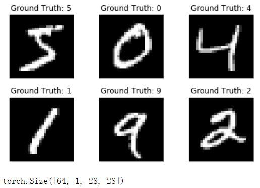
In order to have a more intuitive understanding of MNIST handwritten numeral samples, here we output some samples to have a look
import matplotlib.pyplot as plt

examples = enumerate(trainloader)
batch_idx, (example_data, example_targets) = next(examples)
fig = plt.figure()
for i in range(6):
    plt.subplot(2, 3, i+1)
    plt.tight_layout()
    plt.imshow(example_data[i][0], cmap='gray', interpolation='none')
    plt.title('Ground Truth: {}'.format(example_targets[i]))
    plt.xticks([])
    plt.yticks([])
plt.show()
print(example_data.shape)

Ⅱ. Build network
we need to build a convolutional neural network, which is very suitable for training such image samples with certain spatial position relationship between pixels.
class CNNNet(nn.Module):
    def __init__(self):
        super(CNNNet, self).__init__()
        self.features = nn.Sequential(
            nn.Conv2d(1, 10, kernel_size=3),
            nn.ReLU(),
            nn.MaxPool2d(kernel_size=2, stride=2),
            nn.Conv2d(10, 20, kernel_size=4),
            nn.ReLU(),
            nn.MaxPool2d(kernel_size=2, stride=2)
        )
        self.classifier = nn.Sequential(
            nn.Dropout(),
            nn.Linear(500, 50),
            nn.ReLU(),
            nn.Dropout(),
            nn.Linear(50, 10),
            nn.LogSoftmax(dim=1)
        )
    def forward(self, x):
        x = self.features(x)
        x = torch.flatten(x, 1)
        x = self.classifier(x)
        return x
because our training sample is a gray image with only one channel, the input of the first convolution layer is one dimension, the output is ten dimensions, and the convolution kernel size is 3. The size of the feature image output after the image passes through the first convolution layer is 26 × 26. There are ten dimensions. After passing through the pool layer, the size becomes 13 × 13. After a convolution layer with a convolution kernel size of 4 and a pooling layer, the output characteristic graph size is 5 × 5. There are 20 dimensions in total. At this time, the feature map contains 5 dimensions in total × five × 20 = 500 features.
then, the 500 features are output into 10 dimensions through two full connection layers, that is, the classification results corresponding to 10 numbers from 0 to 9.
Ⅲ. model training
net = CNNNet()

if torch.cuda.is_available():
    device = torch.device('cuda')
else:
    device = torch.device('cpu')
net.to(device)

trainloader, validloader, testloader = get_data()
Before training the model, we need to do several things: 1) define the loss function; 2) Define the optimizer.
# Loss function - cross entropy loss
loss_fn = nn.CrossEntropyLoss()
# Optimizer - Adam optimizer, with a learning rate of 0.01
optimizer = optim.Adam(net.parameters(), lr=0.01)
1. Start training
- Obtain output;
- Gradient clearing;
- Calculate the loss;
- Back propagation;
- parameter optimization
for epoch in range(1, epochs+1):
    model.train()
    for train_idx, (inputs, labels) in enumerate(train_loader, 0):
        inputs = inputs.to(device)
        labels = labels.to(device)
        # 1. Get output
        outputs = model(inputs)
        # 2. Gradient clearing
        optimizer.zero_grad()
        # 3. Calculation of loss
        loss = loss_fn(outputs, labels)
        # 4. Back propagation
        loss.backward()
        # 5. Parameter optimization
        optimizer.step()
        # Print training information
        if train_idx % 10 == 0:
            train_losses.append(loss.item())
            counter_index = train_idx * len(inputs) + (epoch-1) * len(train_loader.dataset)
            train_counter.append(counter_index)
            print('epoch: {}, [{}/{}({:.0f}%)], loss: {:.6f}'.format(
                epoch, train_idx*len(inputs), len(train_loader.dataset), 100*(train_idx*len(inputs)+(epoch-1)*len(train_loader.dataset))/(len(train_loader.dataset)*(epochs)), loss.item()))
2. Model validation
            # validation
            if train_idx % 300 == 0:
                model.eval()
                valid_loss = []
                for valid_idx, (inputs, labels) in enumerate(valid_loader, 0):
                    inputs = inputs.to(device)
                    labels = labels.to(device)
                    outputs = model(inputs)
                    loss = loss_fn(outputs, labels)
                    valid_loss.append(loss.item())
                # Average loss
                valid_losses.append(np.average(valid_loss))
                valid_counter.append(counter_index)
                print('validation loss: {:.6f} counter_index: {}'.format((np.average(valid_loss)), counter_index))
print('training ended')
train(net, optimizer, loss_fn, trainloader, validloader, epochs=2)
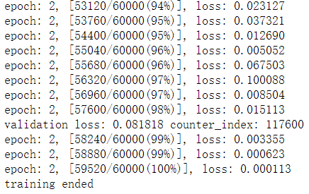
Partial output results

Ⅲ. Model test
# Average test loss
test_loss_avg = 0

def test(model, test_loader, loss_fn, device='cpu'):
    correct = 0
    total = 0
    test_loss = []
    with torch.no_grad():
        for train_idx, (inputs, labels) in enumerate(test_loader, 0):
            inputs = inputs.to(device)
            labels = labels.to(device)
            outputs = net(inputs)
            loss = loss_fn(outputs, labels)
            test_loss.append(loss.item())
            index, value = torch.max(outputs.data, 1)
            total += labels.size(0)
            correct += int((value==labels).sum())
        test_loss_avg = np.average(test_loss)
        print('Total: {}, Correct: {}, Accuracy: {:.2f}%, AverageLoss: {:.6f}'.format(total, correct, (correct/total*100), test_loss_avg))
test(net, testloader, loss_fn)
result
Total: 5000, Correct: 4940, Accuracy: 98.80%, AverageLoss: 0.035709
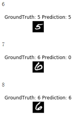
A total of 5000 samples were tested, of which the number of correctly predicted samples was 4940. The following are some prediction results
examples = enumerate(testloader)
batch_idx, (inputs, targets) = next(examples)
with torch.no_grad():
    outputs = net(inputs)
    fig = plt.figure()
    for i in range(0, 50):
        # Among the first 100 test samples, look for samples whose prediction results are inconsistent with the label
        #if(targets[i].item() != outputs.data.max(1, keepdim=True)[1][i].item()):
        print(i)
        plt.subplot(5, 10, i+1)
        plt.imshow(inputs[i][0], cmap='gray', interpolation='none')
        plt.title('GroundTruth: {} Prediction: {}'.format(targets[i], outputs.data.max(1, keepdim=True)[1][i].item()))
        plt.xticks([])
        plt.yticks([])
        plt.show()

You can see that the "6" in the middle is incorrectly predicted as "0"
Ⅳ. Draw image
import matplotlib.pyplot as plt

fig = plt.figure()
plt.plot(train_counter, train_losses, color='blue')
plt.plot(valid_counter, valid_losses, color='red')
plt.scatter(train_counter[-1], test_loss_avg, color='green')
plt.legend(['Train Loss', 'Valid Loss', 'Test Loss'], loc='upper right')
plt.xlabel('Training images number')
plt.ylabel('Loss')
plt.show()

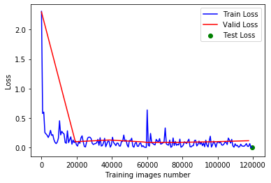
it can be observed from the image that the model training results are good, at least from the results of the verification set, there is no obvious over fitting phenomenon. And the final test results are also ideal.
