Network optimization exercises
0. Overview
Among them, Dropout and Weight Decay are two methods that have been practiced in future experiments (fitting thematic). In this experiment, we will practice some other important network optimization methods.
These include:
(1) Small batch gradient drop (this section will discuss the setup of batch size and learning rate)
(2) Learning Rate Decay
(3) Batch Normalization
(4) Data preprocessing
1. PyTorch library import and dataset introduction
import torch
import torchvision
import torch.nn as nn
import torch.nn.functional as F
import torch.optim as optim

print(torch.manual_seed(1))
<torch._C.Generator object at 0x000001C4DFC45B50>
About datasets:
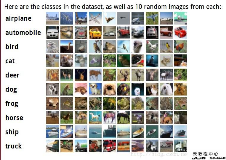
In this experiment, we will use a new image dataset: CIFAR-10. The dataset contains 60,000 RGB color images, of which 50,000 are for training and 10,000 are for testing. Pictures are divided into 10 categories, each with 6,000 pictures, each containing 32*32 pixels.
The sample dataset and 10 categories are as follows:
Official Instructions and Download Address for CIFAR-10: http://www.cs.toronto.edu/~kriz/cifar.html
Compared with previously used MNIST and Fashion-MNIST, the classification of CIFAR-10 is significantly more difficult.
2. Control group results
# training set
batch_size_small = 10  # Small batch: 10 pictures at a time
train_set = torchvision.datasets.CIFAR10('./dataset_cifar10', train=True, download=True,
                                       transform=torchvision.transforms.Compose([
                                           torchvision.transforms.ToTensor(),
                                           torchvision.transforms.Normalize(
                                               (0.4914,0.4822,0.4465), (0.2023,0.1994,0.2010)
                                           )
                                       ])
)

# Test Set
test_set = torchvision.datasets.CIFAR10('./dataset_cifar10', train=False, download=True,
                                      transform=torchvision.transforms.Compose([
                                          torchvision.transforms.ToTensor(),
                                          torchvision.transforms.Normalize(
                                              (0.4914,0.4822,0.4465), (0.2023,0.1994,0.2010)
                                          )
                                      ]))

train_loader_small = torch.utils.data.DataLoader(train_set, batch_size=batch_size_small, shuffle=True)
test_loader_small = torch.utils.data.DataLoader(test_set, batch_size=batch_size_small, shuffle=True)
Files already downloaded and verified
Files already downloaded and verified
A general convolution neural network is designed, which consists of three convolution layers and two fully connected layers.
class CNN5_SmallBatch(nn.Module):
    def __init__(self):
        super(CNN5_SmallBatch, self).__init__()
        self.conv1 = nn.Conv2d(in_channels=3, out_channels=32, padding=1, kernel_size=3)
        self.conv2 = nn.Conv2d(in_channels=32, out_channels=32, padding=1, kernel_size=3)
        self.conv3 = nn.Conv2d(in_channels=32, out_channels=32, padding=1, kernel_size=3)

        self.fc1 = nn.Linear(in_features=32*4*4, out_features=64)
        self.out = nn.Linear(in_features=64, out_features=10)


    def forward(self, t):

        t = self.conv1(t)
        t = F.relu(t)
        t = F.max_pool2d(t, kernel_size=2, stride=2)

        t = self.conv2(t)
        t = F.relu(t)
        t = F.max_pool2d(t, kernel_size=2, stride=2)

        t = self.conv3(t)
        t = F.relu(t)
        t = F.max_pool2d(t, kernel_size=2, stride=2)

        t = t.reshape(batch_size_small, 32*4*4)  # dim0: batch size = 10

        t = self.fc1(t)
        t = F.relu(t)

        t = self.out(t)

        return t
network = CNN5_SmallBatch()
print(network.cuda())
CNN5_SmallBatch(
  (conv1): Conv2d(3, 32, kernel_size=(3, 3), stride=(1, 1), padding=(1, 1))
  (conv2): Conv2d(32, 32, kernel_size=(3, 3), stride=(1, 1), padding=(1, 1))
  (conv3): Conv2d(32, 32, kernel_size=(3, 3), stride=(1, 1), padding=(1, 1))
  (fc1): Linear(in_features=512, out_features=64, bias=True)
  (out): Linear(in_features=64, out_features=10, bias=True)
)
Pre-training preparation
loss_func = nn.CrossEntropyLoss()  # loss function
optimizer = optim.SGD(network.parameters(), lr=0.1)  # Optimizer (learning rate lr equals 0.1)
def get_num_correct(preds, labels):  # get the number of correct times
    return preds.argmax(dim=1).eq(labels).sum().item()
Start training
total_epochs = 10  # Training 10 cycles

for epoch in range(total_epochs):

    total_loss = 0
    total_train_correct = 0

    for batch in train_loader_small:
        images, labels = batch
        images = images.cuda()
        labels = labels.cuda()
        preds = network(images)
        loss = loss_func(preds, labels)

        optimizer.zero_grad()
        loss.backward()
        optimizer.step()

        total_loss += loss.item()
        total_train_correct += get_num_correct(preds, labels)

    print("epoch:", epoch,
          "correct times:", total_train_correct,
          f"training accuracy:", "%.3f" %(total_train_correct/len(train_set)*100), "%",
          "total_loss:", "%.3f" %total_loss)


torch.save(network.cpu(), "cnn5.pt")  # Save Model
epoch: 0 correct times: 20931 training accuracy: 41.862 % total_loss: 8056.230
epoch: 1 correct times: 24131 training accuracy: 48.262 % total_loss: 7359.204
epoch: 2 correct times: 24193 training accuracy: 48.386 % total_loss: 7401.946
epoch: 3 correct times: 24470 training accuracy: 48.940 % total_loss: 7411.769
epoch: 4 correct times: 24225 training accuracy: 48.450 % total_loss: 7540.996
epoch: 5 correct times: 23992 training accuracy: 47.984 % total_loss: 7580.270
epoch: 6 correct times: 24355 training accuracy: 48.710 % total_loss: 7503.453
epoch: 7 correct times: 24148 training accuracy: 48.296 % total_loss: 7539.350
epoch: 8 correct times: 23923 training accuracy: 47.846 % total_loss: 7676.186
epoch: 9 correct times: 23948 training accuracy: 47.896 % total_loss: 7615.532
View test results
network = CNN5_SmallBatch()  # Load Model
network = torch.load("cnn5.pt")

total_test_correct = 0
total_loss = 0

for batch in test_loader_small:
    images, labels = batch
    images = images
    labels = labels
    preds = network(images)
    loss = loss_func(preds, labels)

    total_loss += loss
    total_test_correct += get_num_correct(preds, labels)

print("correct times:", total_test_correct,
      f"test accuracy:", "%.3f" %(total_test_correct/len(test_set)*100), "%",
      "total_loss:", "%.3f" %total_loss)
correct times: 4475 test accuracy: 44.750 % total_loss: 1604.812
3. Small Batch Gradient Decrease: Bach size and learning rate (lr) settings
In the theory lesson, we have learned what small-batch gradient descent is, and we will validate the following conclusions:
- The larger the batch, the smaller the variance of the random gradient, the smaller the noise introduced, and the more stable the training, so a larger learning rate can be set.
- When batches are small, a smaller learning rate needs to be set, otherwise the model will not converge.
(1) To verify the conclusion, we increased the batch size from 10 to 100, keeping the learning rate at 0.1. Observe and discuss the training and test results at this time.
Training results, test results are shown in Fig. 1 and Fig. 2.
[External chain picture transfer failed, source station may have anti-theft chain mechanism, it is recommended to save the picture and upload it directly (img-RGqC0ORr-1643011180639) (C:UsersWatchAppDataRoamingTyporatypora-user-imagesimage-2026.png)]
Figure 1 Training Result (batch size=100, lr=0.1)
[External chain picture transfer failed, source station may have anti-theft chain mechanism, it is recommended to save the picture and upload it directly (img-HMvInVBA-1643011180639) (C:UsersWatchAppDataRoamingTyporatypora-user-imagesimage-2016262626;6.png)]
Figure 2 Test Results (batch size=100, lr=0.1)
Compared with the control group, we found that the accuracy of network testing increased from about 42% to about 71%, with a significant improvement. The reason is that maintaining the same learning rate ensures that the optimization algorithm takes the same step size each time. Increasing the batch size optimization algorithm yields more loss information so that it can move in a more correct direction (global or local minimum). With the same size of steps and more accurate direction, you will get better training results in a limited training cycle, and the test results will naturally be better. So a large batch size corresponds to a large learning rate.
4. Learning Rate Decay
Generally speaking, we want to have a higher learning rate at the beginning of training, make the network converge quickly, and a smaller learning rate at the end of training, so that the network can converge to the optimal solution better.
Let's do the following: Keep the batch size at 10, and at the end of each cycle, the learning rate decays by 0.8 times as much. Observe and discuss the training and test results at this time.
The training results are shown in Figure 3 and the test results are shown in Figure 4.
[External chain picture transfer failed, source station may have anti-theft chain mechanism, it is recommended to save the picture and upload it directly (img-HIP5miTW-1643011180640) (C:UsersLook atAppDataRoamingTyporatypora-user-imagesimage-2029.png)]
Figure 3 Training results (learning rate decay)
[External chain picture transfer failed, source station may have anti-theft chain mechanism, it is recommended to save the picture and upload it directly (img-EibK8Nw4-1643011180640) (C:UsersWatchAppDataRoamingTyporatypora-user-imagesimage-202117.png)]
Figure 4 Test Results (Learning Rate Decay)
Compared with the control group, we found that the accuracy of network testing increased from about 42% to about 71%, with a significant improvement. The reason is that at the beginning of the study, you are usually far from the minimum, so take a larger step with a larger learning rate to speed up the training. However, as the training proceeds, it is close to the minimum value, so the learning rate is smaller, which makes the network converge to the optimal solution better.
In addition to reducing learning rates manually, PyTorch also provides us with a variety of learning rate decay strategies. Interested students can read the instructions "How to adjust learning rate" on the official website. https://pytorch.org/docs/stable/optim.html).
5. Batch Normalization
Batch normalization method has been widely used in neural networks, and it has many significant advantages, such as the ability to effectively improve network generalization, the ability to choose a larger initial learning rate, and the ability to improve network convergence.
Interested students can refer to the following:'Batch Normalization: Accelerating Deep Network Training by Reducing Internal Covariate Shift'
Next, while maintaining the batch size (10) and learning rate (0.1), we redefine and train a convolution neural network containing the batch normalization layer (nn.BatchNorm2d). Please observe and discuss the training and test results.
# ------------- data loader (batch size = 10) -------------
# Use train_loader_small and test_loader_small


# ------------- network (including batch normalization processing) -------------
class CNN5_BatchNorm(nn.Module):
    def __init__(self):
        super(CNN5_BatchNorm, self).__init__()
        self.conv1 = nn.Conv2d(in_channels=3, out_channels=32, padding=1, kernel_size=3)
        self.bn1 = nn.BatchNorm2d(32)  # Batch Normalization Layer (32: Number of Input Channels)
        self.conv2 = nn.Conv2d(in_channels=32, out_channels=32, padding=1, kernel_size=3)
        self.bn2 = nn.BatchNorm2d(32)  # Batch Normalization Layer (32: Number of Input Channels)
        self.conv3 = nn.Conv2d(in_channels=32, out_channels=32, padding=1, kernel_size=3)
        self.bn3 = nn.BatchNorm2d(32)  # Batch Normalization Layer (32: Number of Input Channels)

        self.fc1 = nn.Linear(in_features=32*4*4, out_features=64)
        self.out = nn.Linear(in_features=64, out_features=10)


    def forward(self, t):

        t = self.conv1(t)  # conv1
        t = self.bn1(t)  # batch normalization
        t = F.relu(t)
        t = F.max_pool2d(t, kernel_size=2, stride=2)

        t = self.conv2(t)  # conv2
        t = self.bn2(t)  # batch normalization
        t = F.relu(t)
        t = F.max_pool2d(t, kernel_size=2, stride=2)

        t = self.conv3(t)  # conv3
        t = self.bn3(t)  # batch normalization
        t = F.relu(t)
        t = F.max_pool2d(t, kernel_size=2, stride=2)

        t = t.reshape(batch_size_small, 32*4*4)

        t = self.fc1(t)  # fc1
        t = F.relu(t)

        t = self.out(t)  # output layer

        return t


network = CNN5_BatchNorm()
network.cuda()


# -------------- Training-----------------
optimizer = optim.SGD(network.parameters(), lr=0.1)  # The learning rate lr is set to 0.1

for epoch in range(total_epochs):

    total_loss = 0
    total_train_correct = 0

    for batch in train_loader_small:
        images, labels = batch
        images = images.cuda()
        labels = labels.cuda()
        preds = network(images)
        loss = loss_func(preds, labels)

        optimizer.zero_grad()
        loss.backward()
        optimizer.step()

        total_loss += loss.item()
        total_train_correct += get_num_correct(preds, labels)

    print("epoch:", epoch,
          "correct times:", total_train_correct,
          f"training accuracy:", "%.3f" %(total_train_correct/len(train_set)*100), "%",
          "total_loss:", "%.3f" %total_loss)


torch.save(network.cpu(), "cnn5.pt")  # Save Model
The training results are shown in Figure 5 and the test results are shown in Figure 6.
[External chain picture transfer failed, source station may have anti-theft chain mechanism, it is recommended to save the picture and upload it directly (img-QtARMlIx-1643011180641) (C:UsersLook atAppDataRoamingTyporatypora-user-imagesimage-2023.png)]
Figure 5 Training Results (Batch Normalization)
[External chain picture transfer failed, source station may have anti-theft chain mechanism, it is recommended to save the picture and upload it directly (img-DYDAuZQa-1643011180641) (C:UsersWatchAppDataRoamingTyporatypora-user-imagesimage-20202220.png)]
Figure 6 Test Results (Batch Normalization)
Compared with the control group, we found that the accuracy of network testing increased from about 42% to about 73%, with a significant improvement. The reason is that in deep neural networks, the middle input is the output of the previous one. As a result, changes in the parameters of the previous layer's neural network can result in large differences in the distribution of inputs at the current layer. When a random gradient descent method is used to train a neural network, each parameter update results in a change in the input distribution at each level of the network. The deeper the neural network is, the more obvious the distribution of its inputs will change. From a machine learning perspective, if the input distribution of a layer changes, its parameters need to be relearned, a phenomenon called internal covariant offset. In order to solve the internal covariate offset problem, it is necessary to make the distribution of each layer of neural network input consistent during training. The easiest way is to normalize each layer of the neural network so that its distribution remains stable. Batch normalization can make the input distribution of each layer of the neural network keep consistent during the training process, so it can effectively improve the network performance.
6. Data Preprocessing
In previous experiments, we standardized the data each time before transferring it to a neural network. Next, we cancel the standardization and shuffle settings and set the batch size and learning rate to 100 and 0.1, respectively. Please compare them with 3-(1) to see if data preprocessing affects the results.
# ------------- data loader (batch size = 100, cancel standardization) ---------------
train_set_noTransform = torchvision.datasets.CIFAR10('./dataset_cifar10', train=True, download=True,
                                                     transform=torchvision.transforms.Compose([
                                                         torchvision.transforms.ToTensor(),
                                                     ]))
test_set_noTransform = torchvision.datasets.CIFAR10('./dataset_cifar10', train=False, download=True,
                                                    transform=torchvision.transforms.Compose([
                                                        torchvision.transforms.ToTensor(),
                                                    ]))
The training results are shown in Figure 7 and the test results are shown in Figure 8.
[External chain picture transfer failed, source station may have anti-theft chain mechanism, it is recommended to save the picture and upload it directly (img-xcFMMLqn-1643011180642) (C:UsersLook atAppDataRoamingTyporatypora-user-imagesimage-2022.png)]
Figure 7 Training Results (batch size=100, lr=0.1, no pre-processing)
[External chain picture transfer failed, source may have anti-theft chain mechanism, it is recommended to save the picture and upload it directly (img-4pUHemMh-1643011180642) (C:UsersLook atAppDataRoamingTyporatypora-user-imagesimage-201013.png)]
Figure 8 test results (batch size=100, lr=0.1, no preprocessing)
Compared with the group with "batch size=100, lr=0.1, with pretreatment", we found that the accuracy of network testing decreased from about 71% to about 65%, with a significant decrease. Analysis Reason: Adding preprocessing can make the input data in a better distribution, which is more conducive to the training of the network, and make the optimization algorithm easier to find the optimal solution direction and faster convergence.