Catalogue of series articles

PyTorch Week 3 - nn.MaxPool2d, nn.AvgPool2d, nn.Linear, active layer
PyTorch Week 3 - convolution
PyTorch Week 3 -- container of nn.Module: Sequential, ModuleList, ModuleDice
PyTorch Week 3 - model creation
PyTorch Week 2 - Dataloader and Dataset
PyTorch Week 1

preface

In this section, the principle of gradient disappearance and gradient explosion is understood through code and formula derivation, as well as the solution by initializing the weight.

1, Gradient disappearance and gradient explosion

1. The causes of gradient disappearance and explosion are analyzed by formula derivation

Regardless of the activation function and deviation, explore the impact of weight initialization on the output

Demonstrate the gradient explosion caused by the output of the previous layer

Take three linear layers as an example:

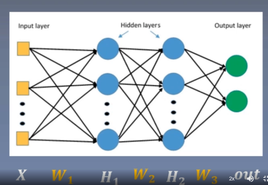
Suppose we ask for the gradient of W2:

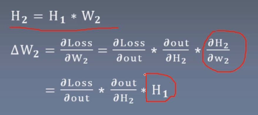
It can be seen that the gradient of W2 is affected by the input H1 of the previous layer. If H1 approaches 0, the gradient of W2 disappears. If H1 approaches infinity, the gradient of W2 explodes
Code demonstration
A 100 layer model with 256 units in each layer is constructed. The weight of each layer is initialized by standard normal distribution, mean=0, std=1. The input is also normal: mean=0, std=1

class MLP(nn.Module):
    def __init__(self, neural_num, layers):
        super(MLP, self).__init__()
        self.linears = nn.ModuleList([nn.Linear(neural_num, neural_num, bias=False) for i in range(layers)])#Building ModuleList model by list derivation
        self.neural_num = neural_num
        
    def forward(self, x):
        for (i, linear) in enumerate(self.linears):
            x = linear(x)
        return x
        
    def initialize(self):
        for m in self.modules():
            if isinstance(m, nn.Linear):
                nn.init.normal_(m.weight.data)#Initialization of standard normal distribution, mean=0, std=1
                
layer_nums = 100
neural_nums = 256
batch_size = 16

net = MLP(neural_nums, layer_nums)#A 100 layer model with 256 units in each layer is constructed
net.initialize() #
inputs = torch.randn((batch_size, neural_nums))  # normal: mean=0, std=1
output = net(inputs)
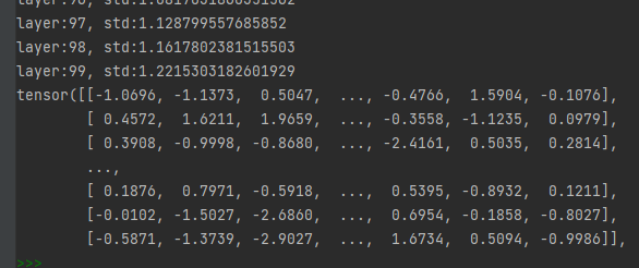
print(output)

Printout, explosion.

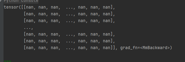
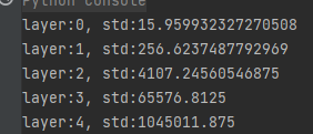
Let's measure the distribution range of output data of each layer by standard deviation, and find out which layer's output starts to explode

Formula derivation explores the reasons for the increasing output of each layer

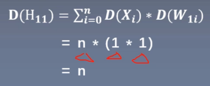
Regardless of bias, if the standard deviation of X*Y = the product of the standard deviation of X and Y, the variance of output H11 of layer 11 = n × (variance of x) × (W) During initialization, the input and the weight of each layer are the mean value 0 and the standard deviation is 1 (variance is 1). Therefore, the standard deviation of the output of the first unit of layer 1 is n under the root sign and N times under the expanded root sign of each layer

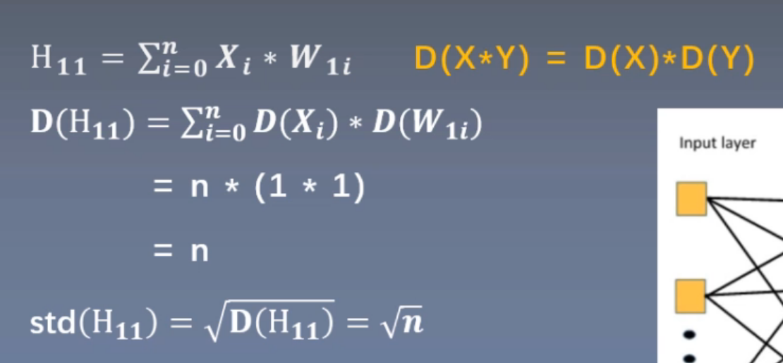
When the number of the first layer is 256, the standard deviation is about 16, the second layer is expanded 16 times, and the standard deviation is 256, and so on. The code verification is consistent with the expected performance

Formula derivation to explore the method of alleviating gradient explosion

As shown in the figure below, as long as the output variance of each layer is guaranteed to be 1


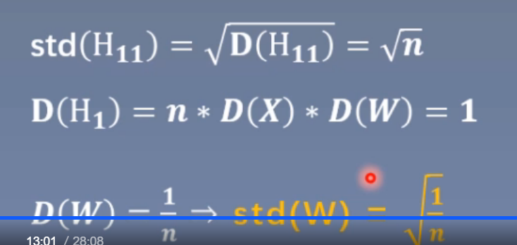
Then, in order to ensure that the variance of the output is equal to 1, just let the standard deviation of the weight = under the root sign (1/n).

Code verification

nn.init.normal_(m.weight.data, std=np.sqrt(1/self.neural_num))#

It can be seen that the output of each layer is still maintained in a small range.

2, Consider the influence of activation function

1.Xavier initialization

formula

reference: <Understanding the difficulty of training deep feedforward neural networks>
Objective: variance consistency, that is to maintain the data scale (network output value of each layer) in an appropriate range, usually the variance is 1
Activation function for: saturation function, such as Sigmoid, Tanh

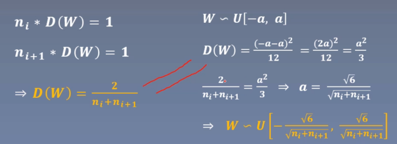
In order to satisfy the variance consistency, the variance of the weight should satisfy the left formula.
The weight generally satisfies the uniform distribution. In order to ensure that the mean value is 0 and the upper and lower limits of the uniform distribution are opposite to each other, set the upper limit as a, then the variance of the weight should meet the third a square and make it equal to the left formula, then the weight initialization should meet the right formula.

code

First, add the activation function layer, and then modify the weight initialization method

    def forward(self, x):
        for (i, linear) in enumerate(self.linears):
            x = linear(x)
            x = torch.tanh(x)#Add tanh layer
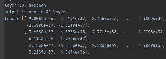
            print("layer:{}, std:{}".format(i, x.std()))
            if torch.isnan(x.std()):
                print("output is nan in {} layers".format(i))
                break
        return x

    def initialize(self):
        for m in self.modules():
            if isinstance(m, nn.Linear):
                a = np.sqrt(6 / (self.neural_num + self.neural_num))#Calculate uniform Distributiona
                tanh_gain = nn.init.calculate_gain('tanh')#Using nn.init.calculate_gain obtains the a gain of each layer
                a *= tanh_gain#Calculate a for each layer
                nn.init.uniform_(m.weight.data, -a, a)#Weight initialization

Still maintain a small value

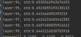
Pytorch also provides nn.init.xavier_uniform_(m.weight.data, gain=tanh_gain) method is used to realize the same function

tanh_gain = nn.init.calculate_gain('tanh')
nn.init.xavier_uniform_(m.weight.data, gain=tanh_gain)

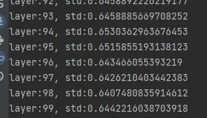
Completely consistent

2.Kaiming initialization method

reference Delving Deep into Rectifiers: Surpassing Human-Level Performance on ImageNet Classification

formula

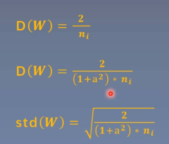
Variance consistency
Function for: ReLU function and its variants
After formula derivation, the variance and standard deviation of the weight shall be:

code

The activation function is changed to:

x = torch.relu(x)

Change initialization to:

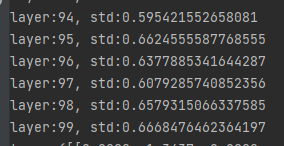
nn.init.normal_(m.weight.data, std=np.sqrt(2 / self.neural_num))

result

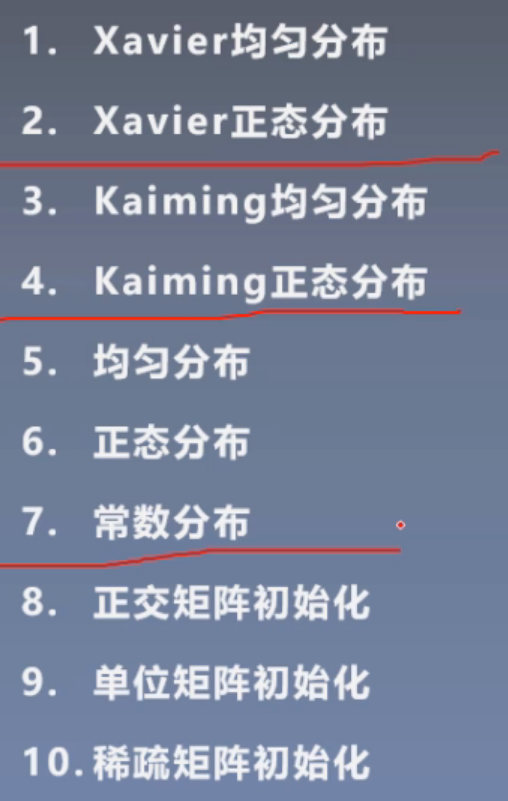
3, Ten initialization methods

summary

• From the perspective of formula derivation, it is understood that the reason for gradient disappearance and gradient explosion is the output of each layer
• By deriving the variance formula of the output of each layer, it is analyzed that the variance of the output layer is related to the number of neurons, the variance of the input and the variance of the weight; The weight initialization variance is 1, which can effectively suppress the gradient disappearance and gradient explosion.
• There are different initialization methods for different activation functions. Xavier initialization is for saturation function and Kaiming initialization is for ReLU and its variants.