Original link: http://tecdat.cn/?p=3385
Original source: Tuo end data tribal official account
Recently, I was asked to write a copulas survey on financial time series. Obtain the description of various models from the read data, including some graphics and statistical output.
> oil = read.xlsx(temp,sheetName ="DATA",dec =",")
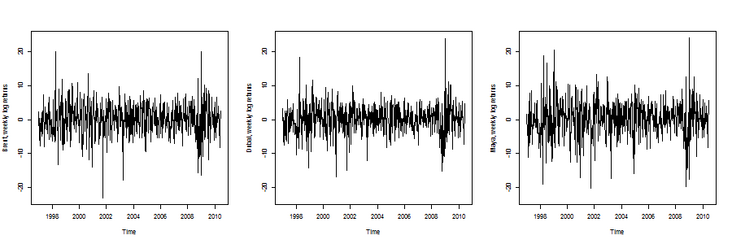
Then we can draw these three time series
1 1997-01-10 2.73672 2.25465 3.3673 1.5400

2 1997-01-17 -3.40326 -6.01433 -3.8249 -4.1076

3 1997-01-24 -4.09531 -1.43076 -6.6375 -4.6166

4 1997-01-31 -0.65789 0.34873 0.7326 -1.5122

5 1997-02-07 -3.14293 -1.97765 -0.7326 -1.8798

6 1997-02-14 -5.60321 -7.84534 -7.6372 -11.0549
The idea is to use some multivariable ARMA-GARCH processes here. The heuristic here is that the first part is used to simulate the dynamics of time series mean value, and the second part is used to simulate the dynamics of time series variance.
Two models are considered in this paper
- Multivariable GARCH process on ARMA model residuals (or variance matrix dynamic model)
- Multivariable model of ARMA-GARCH process residuals (based on copula)
Therefore, different sequences will be considered here and obtained as residuals of different models. We can also standardize these residuals.
ARMA model
> fit1 = arima(x = dat \[,1\],order = c(2,0,1))
> fit2 = arima(x = dat \[,2\],order = c(1,0,1))
> fit3 = arima(x = dat \[,3\],order = c(1,0,1))
> m < - apply(dat_arma,2,mean)
> v < - apply(dat_arma,2,var)
> dat\_arma\_std < - t((t(dat_arma)-m)/ sqrt(v))
ARMA-GARCH model
> fit1 = garchFit(formula = ~arma(2,1)+ garch(1,1),data = dat \[,1\],cond.dist ="std")
> fit2 = garchFit(formula = ~arma(1,1)+ garch(1,1),data = dat \[,2\],cond.dist ="std")
> fit3 = garchFit(formula = ~arma(1,1)+ garch(1,1),data = dat \[,3\],cond.dist ="std")
> m\_res < - apply(dat\_res,2,mean)
> v\_res < - apply(dat\_res,2,var)
> dat\_res\_std = cbind((dat\_res \[,1\] -m\_res \[1\])/ sqrt(v\_res \[1\]),(dat\_res \[,2\] -m\_res \[2\])/ sqrt(v\_res \[2\]),(dat\_res \[ ,3\] -m\_res \[3\])/ SQRT(v_res \[3\]))
Multivariable GARCH model
The first model that can be considered is multivariable EWMA of covariance matrix,
> ewma = EWMAvol(dat\_res\_std,lambda = 0.96)
Volatility
> emwa\_series\_vol = function(i = 1){
+ lines(Time,dat_arma \[,i\] + 40,col ="gray")
+ j = 1
+ if(i == 2)j = 5
+ if(i == 3)j = 9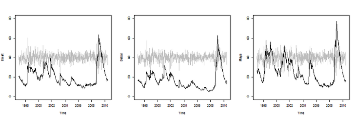
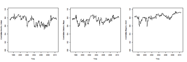
Implicit correlation
> emwa\_series\_cor = function(i = 1,j = 2){
+ if((min(i,j)== 1)&(max(i,j)== 2)){
+ a = 1; B = 9; AB = 3}
+ r = ewma $ Sigma.t \[,ab\] / sqrt(ewma $ Sigma.t \[,a\] *
+ ewma $ Sigma.t \[,b\])
+ plot(Time,r,type ="l",ylim = c(0,1))
+}
Multivariable GARCH, i.e. BEKK (1,1) model, for example:
> bekk = BEKK11(dat_arma)
> bekk\_series\_vol function(i = 1){
+ plot(Time, $ Sigma.t \[,1\],type ="l",
+ ylab = (dat)\[i\],col ="white",ylim = c(0,80))
+ lines(Time,dat_arma \[,i\] + 40,col ="gray")
+ j = 1
+ if(i == 2)j = 5

+ if(i == 3)j = 9

> bekk\_series\_cor = function(i = 1,j = 2){
+ a = 1; B = 5; AB = 2}
+ a = 1; B = 9; AB = 3}
+ a = 5; B = 9; AB = 6}
+ r = bk $ Sigma.t \[,ab\] / sqrt(bk $ Sigma.t \[,a\] *
+ bk $ Sigma.t \[,b\])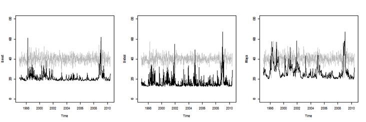
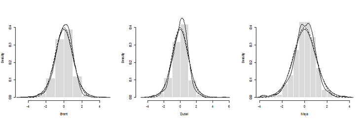
Simulating residuals from univariate GARCH model
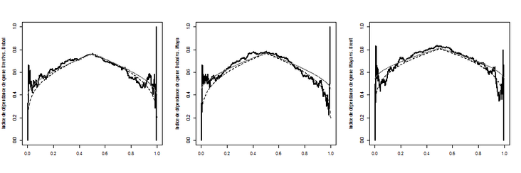
The first step may be to consider some static (joint) distributions of residuals. Univariate marginal distribution is
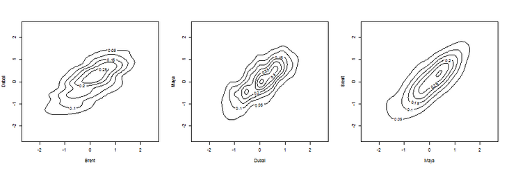
Contour of edge density (obtained using bivariate kernel estimator)
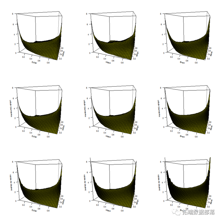
The density of Copula can also be visualized (there are some nonparametric estimates above and parametric copula below)
> copula_NP = function(i = 1,j = 2){
+ n = nrow(uv)
+ s = 0.3

+ norm.cop < - normalCopula(0.5)
+ norm.cop < - normalCopula(fitCopula(norm.cop,uv)@estimate)
+ dc = function(x,y)dCopula(cbind(x,y),norm.cop)


+ ylab = names(dat)\[j\],zlab ="copule Gaussienne",ticktype ="detailed",zlim = zl)
+
+ t.cop < - tCopula(0.5,df = 3)
+ t.cop < - tCopula(t.fit \[1\],df = t.fit \[2\])


+ ylab = names(dat)\[j\],zlab ="copule de Student",ticktype ="detailed",zlim = zl)
+}
You can consider this Function,
Calculate the empirical versions of the three sequences and compare them with some parameter versions,
>

> lambda = function(C){
+ l = function(u)pcopula(C,cbind(u,u))/ u
+ v = Vectorize(l)(u)
+ return(c(v,rev(v)))
+}
>

> graph_lambda = function(i,j){
+ X = dat_res
+ U = rank(X \[,i\])/(nrow(X)+1)
+ V = rank(X \[,j\])/(nrow(X)+1)

+ normal.cop < - normalCopula(.5,dim = 2)
+ t.cop < - tCopula(.5,dim = 2,df = 3)
+ fit1 = fitCopula(normal.cop,cbind(U,V),method ="ml")
d(U,V),method ="ml")
+ C1 = normalCopula(fit1 @ copula @ parameters,dim = 2)
+ C2 = tCopula(fit2 @ copula @ parameters \[1\],dim = 2,df = trunc(fit2 @ copula @ parameters \[2\]))
+
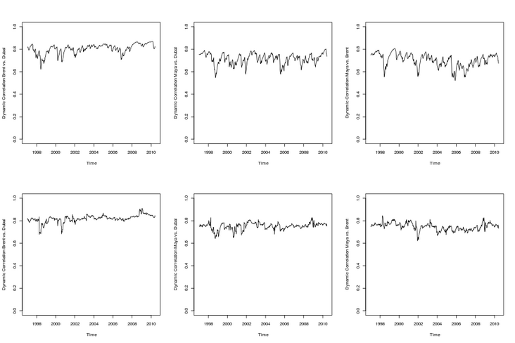
But one may wonder whether the correlation is stable over time.
> time\_varying\_correl_2 = function(i = 1,j = 2,
+ nom_arg ="Pearson"){
+ uv = dat_arma \[,c(i,j)\]
nom_arg))\[1,2\]
+}
> time\_varying\_correl_2(1,2)
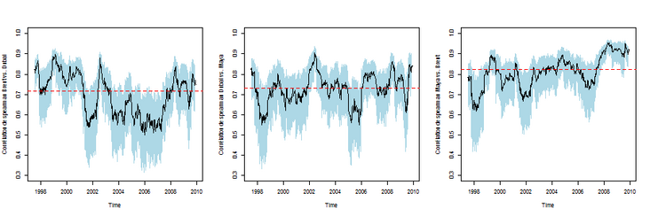
> time\_varying\_correl_2(1,2,"spearman")
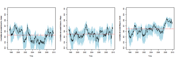
> time\_varying\_correl_2(1,2,"kendall")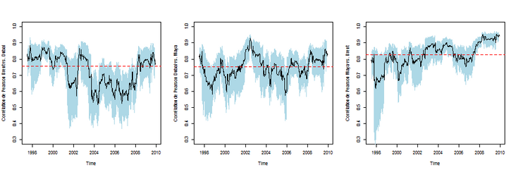
Correlation coefficient between Spearman and time-varying ranking
Or Kendall correlation coefficient
DCC model (S) is considered for the relevance of the model
> m2 = dccFit(dat\_res\_std)
> m3 = dccFit(dat\_res\_std,type ="Engle")
> R2 = m2 $ rho.t
> R3 = m3 $ rho.t
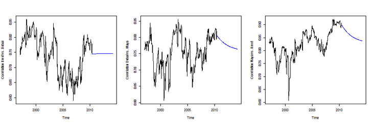
To get some predictions, use, for example
> garch11.spec = ugarchspec(mean.model = list(armaOrder = c(2,1)),variance.model = list(garchOrder = c(1,1),model ="GARCH"))
> dcc.garch11.spec = dccspec(uspec = multispec(replicate(3,garch11.spec)),dccOrder = c(1,1),
distribution ="mvnorm")
> dcc.fit = dccfit(dcc.garch11.spec,data = dat)
> fcst = dccforecast(dcc.fit,n.ahead = 200)

Most popular insights
2.HAR-RV model based on mixed data sampling (MIDAS) regression in R language to predict GDP growth Regressive HAR-RV model predicts GDP growth ")
3.Realization of Volatility: ARCH model and HAR-RV model
5.VaR comparison of GARCH (1,1), MA and historical simulation method
6.R language multivariate COPULA GARCH model time series prediction
7.VAR fitting and prediction based on ARMA-GARCH process in R language
8.matlab predicts ARMA-GARCH conditional mean and variance model
9.ARIMA + GARCH trading strategy for S & P500 stock index in R language