Random number generator of Gaussian distribution
The implementation process is to first find the blog of the implementation of relevant Gaussian random numbers in vivado, first get a general understanding, and then go to HowNet to find the relevant master's thesis, summarize the simplest implementation method of Gaussian random number generation, and carry out simulation verification.
After consulting relevant papers, the Gaussian distribution random number generator is divided into two modules:
Module 1: generate uniform random number based on cellular automata. Specifically, the uniform random number generator of 64 order cellular automata is used to generate uniform random number.
Module 2: convert uniform random number into Gaussian random number through box Muller algorithm.
Module 1: generating uniform random numbers by cellular automata
The earliest idea of cellular automata originated from Stanislaw Ulam, which is a special finite state machine with discreteness of time, space and state. Due to the complexity of the concept of cellular automata, the early research on cellular automata basically focused on the theoretical aspect. Until the early 1980s, S. wolfram 46 first simplified the concept of cellular automata, which greatly promoted the research of cellular automata mechanism theory and its application. Cellular automata is an array composed of a group of cell units in D-dimensional space. A cellular automata can be expressed as four tuples:
Among them, spatial structure A is A spatial structure composed of D-dimensional cell units, and state space -q is the value range of state of cell unit i in cellular automata; The neighborhood function rule is the mapping between the 0-order neighborhood state configuration of the ith cell unit determined by the neighborhood radius r of cellular automata and its transition state: boundary condition B specifies the treatment method of the neighborhood unit within the domain radius of A cell unit when it exceeds the spatial structure of cellular automata.
The code implements the uniform random number generator of 32-order cellular automata to generate uniform random numbers. By giving the initial value and rule number of 32-bit cells (rule 90 and rule 150), instantiating a single cell 32 times, we can get 32-bit cellular automata.
Individual cells are as follows
 module single_cell#(parameter init = 1'b0 , head = 1'b0, tail = 1'b0)
(
input clk_i,rst_n_i,
input ctrl,
input self,left,right,

output out
);

reg  self_next;

always @(*) begin
    case({head,tail})
             2'b10 : self_next = ctrl ? self ^ right : right;
             2'b01 : self_next = ctrl ? self ^ left  : left;
             2'b00 : self_next = ctrl ? left ^ self ^ right : left ^ right;
             default:  self_next = ctrl ? left ^ self ^ right : left ^ right;
    endcase
end

assign out = self_next;

endmodule
Instantiation process: because there is a difference between head and tail cells and intermediate cells, they are divided into three parts. Take the intermediate cells as an example, just change left (uni_r [I-1]) to left (1'b0), which is the head cells right (uni_r[i+1]) is changed to right (1'b0) is the tail cell
module mata
  #(parameter INTA_VEC = 32'b0100_1000_0001_0010_0100_1000_0001_0010,
    parameter RULE_VEC   = 32'b0000_1100_0100_0111_0000_1100_0000_0110,
    N = 32   )

   (
     input clk_i,rst_n_i,
     input pause_i,        //suspend
     output [N-1:0] out_1  //Uniform random number
   );

  reg  [N-1:0] uni_r;
  wire [N-1:0] uni_next;
  assign out_1 = uni_r;

  always @(posedge clk_i or negedge rst_n_i)
  begin
    if(~rst_n_i)
      uni_r <= INTA_VEC;
    else if(pause_i)
      uni_r <= uni_r;
    else
      uni_r <= uni_next;
  end

  generate
    genvar i;
    for (i = 0; i < N; i = i + 1 )
    begin
      if( i==0 )
      begin//first place
        single_cell
          #(.init (INTA_VEC[i]),.head(1'b1 ),.tail (1'b0))
          single_cell_first_num (
            .clk_i (clk_i ),
            .rst_n_i (rst_n_i ),
            .ctrl (RULE_VEC[i] ),
            .left ( 1'b0),
            .right (uni_r[1]),
            .self (uni_r[i]),
            .out  ( uni_next[i])
          );
      end

      else if(i == N - 1)
      begin//Last
        single_cell
          #(.init (INTA_VEC[i] ),.head(1'b0 ),.tail (1'b1))
          single_cell_num (
            .clk_i (clk_i ),
            .rst_n_i (rst_n_i ),
            .ctrl (RULE_VEC[i] ),
            .left ( uni_r[i-1]),
            .right (1'b0),
            .self (uni_r[i]),
            .out  ( uni_next[i])
          );
      end


      else
      begin //Median
        single_cell
          #(.init (INTA_VEC[i] ),.head(1'b0 ),.tail (1'b0))
          single_cell_mid_num (
            .clk_i (clk_i ),
            .rst_n_i (rst_n_i ),
            .ctrl (RULE_VEC[i] ),
            .left ( uni_r[i-1]),
            .right (uni_r[i+1]),
            .self (uni_r[i]),
            .out  ( uni_next[i])
          );
      end
    end
  endgenerate

endmodule
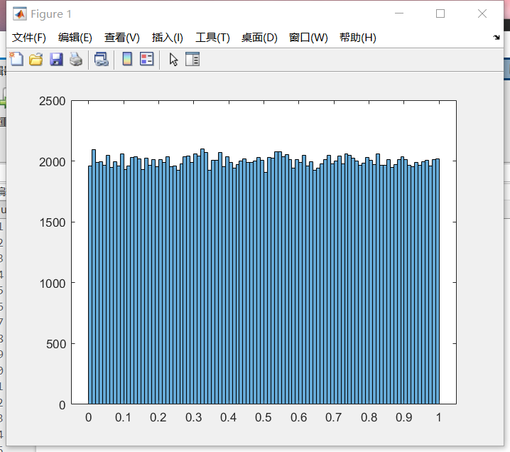
The 32 order cellular automata is simulated
Give the initial value and rule number of 32-bit cells, give the timing clock, collect data and write it into new_data_b.txt text to facilitate the next simulation on matlab.
module tb_celluar_auto();
  // Parameters
  localparam  INTA_VEC = 32'b0100_1000_0001_0010_0100_1000_0001_0010;
  localparam  RULE_VEC = 32'b0000_1100_0100_0111_0000_1100_0000_0110;

  localparam  N = 32;
  localparam  period = 10; //100Mhz

  // Ports
  reg clk_i = 0;
  reg rst_n_i = 1;
  reg pause_i = 0;
  wire [N-1:0] out_1;

  mata
  #(
    .INTA_VEC(INTA_VEC ),
    .RULE_VEC(RULE_VEC ),
    .N (N)
  )
  mata_dut (
    .clk_i (clk_i ),
    .rst_n_i (rst_n_i ),
    .pause_i (pause_i ),
    .out_1  ( out_1)
  );

parameter M = 200_000;
reg [N-1:0] men [M:1];
integer index = 1;
initial begin //reset
    begin
      #(period*2) rst_n_i = 1'b0;
      #(period*10) rst_n_i = 1'b1;

      #(period*201_000);
      $writememb("new_data_b.txt",men);
      $finish;
    end
  end

  initial //Collect data
    begin
        #(period*100);
        forever begin
            #(period);
            men[index] = out_1;
            index = (index >= M) ? 1 : index + 1;
        end
    end

  always //Generate clock
    #(period)  clk_i = ! clk_i ;

endmodule
Simulation results: by importing txt text data into matlab, we can see that the simulation results basically conform to the uniform distribution between 0 and 1.
At the end of module 1, we will proceed to module 2, box Muller algorithm
Box Muller algorithm is one of the earliest algorithms to generate Gaussian white noise. It uses uniform random numbers to calculate the amplitude and phase values of Gaussian random numbers respectively, so as to generate Gaussian random numbers. Box Muller algorithm can convert two uniform random numbers into two Gaussian random numbers at the same time. The underlying principle is very profound, but the result is quite simple. Assuming that X and X are independent Gaussian random variables with zero mean and subject to standard normal distribution, R = √ x2+x20=arctan(x2/x) obey Rayleigh distribution and uniform distribution respectively. Using this fact, a pair of Gaussian variables can be generated by transforming a pair of random variables subject to Rayleigh distribution and a pair of random variables subject to uniform distribution. The specific algorithm is as follows:
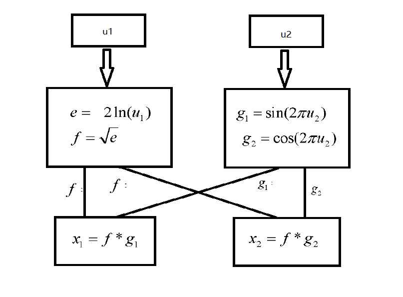
Where u1 and u2 are uniformly distributed random variables on [01], u is used to generate the amplitude value of Gaussian random number, and u is used to generate the phase value of Gaussian random number. Because the algorithm involves logarithmic function and trigonometric function, we use matlab to generate the trigonometric function value of the corresponding variable, store it in the IP core of ROM in vivado, and then get the calculation result of the corresponding function through the look-up table. The logarithmic function is directly added to the IP core in vivado.
Select single ended input rom
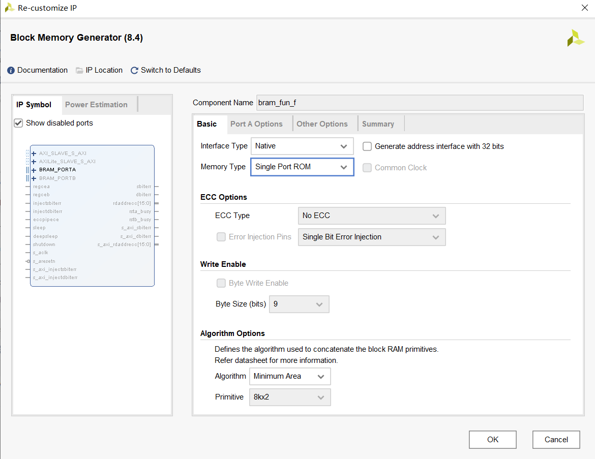
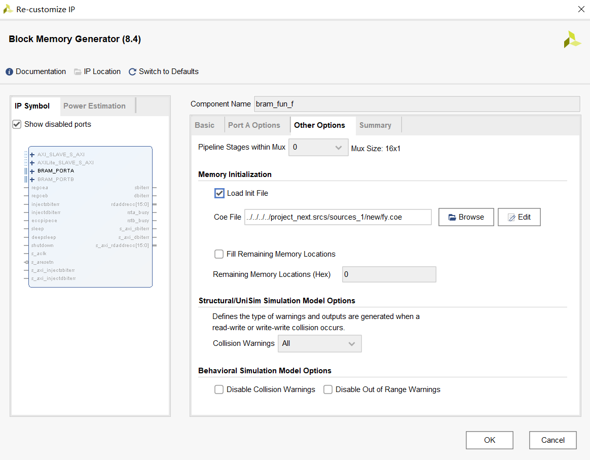
The coe file generated by matlab is imported into the rom ip core, and the ip core is named.
Add an ip core of logarithmic function
Failed to save the image directly to the external link (t4-89939393939393939393939393939393939393c-image) (it is recommended to upload the image directly to the external link)
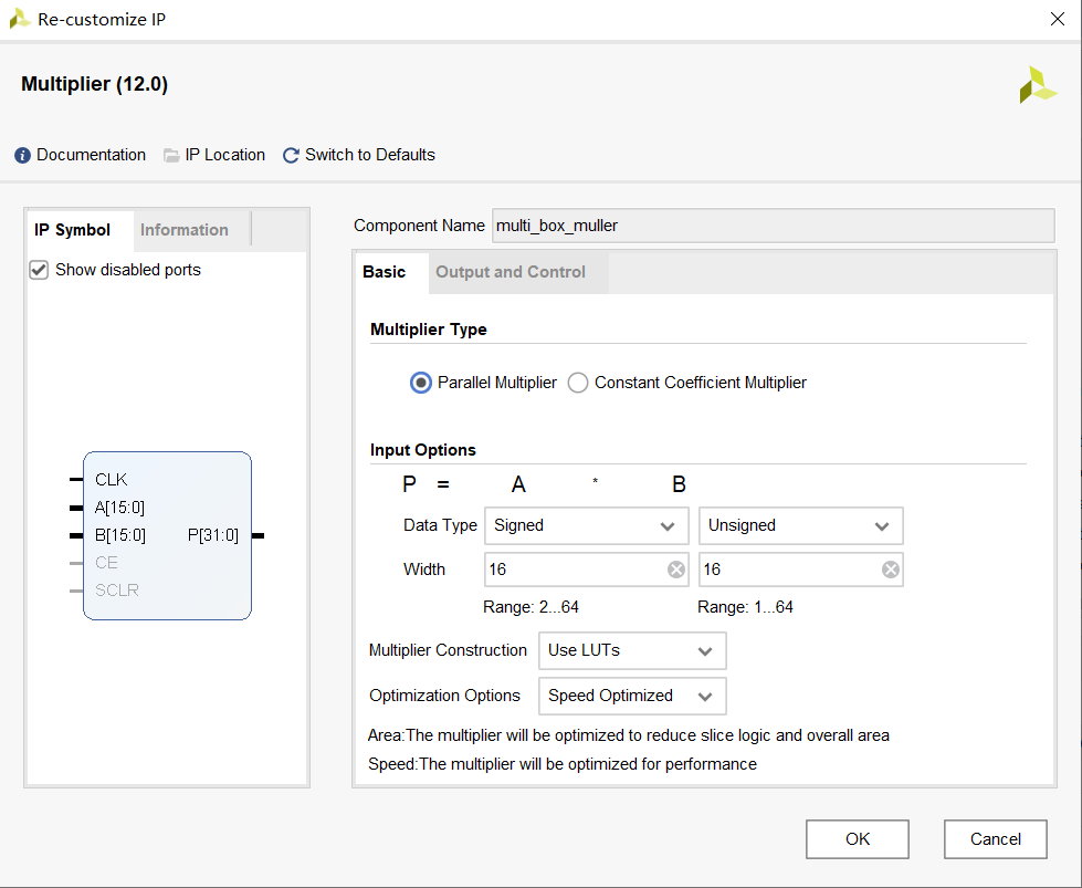
Next, add the ip core of the multiplier and name it.
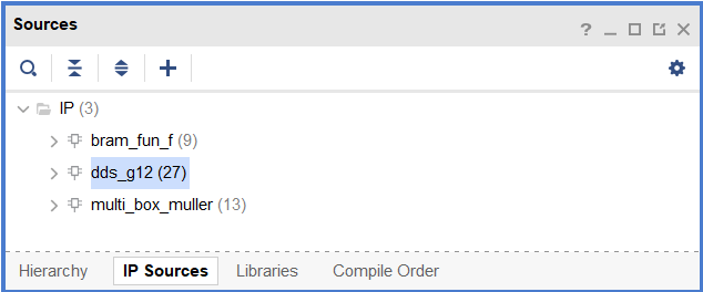
You can see the added ip core in IP Sources
Instantiate the ip core and complete the box Muller algorithm.
module box_muller(
  input clk_i ,rst_n_i,//reset
  input [63:0] uni_i,

  output [31:0] gau1_o,
  output [31:0] gau2_o
    );

    wire [15:0] uni_g= uni_i [63:48];
    wire [15:0] uni_f= uni_i [31:16];
    wire [15:0] fun_f_o;
    wire [15:0] g1_sin_o;
    wire [15:0] g2_cos_o;
    wire m_axis_data_tvalid;
    //wire [15:0] g1_sin_o,g2_cos_o;

  dds_g12 dds_g12_inst (
  .aclk(clk_i),                                // input wire aclk
  .aresetn(rst_n_i),                          // input wire aresetn
  .s_axis_phase_tvalid(1'b1),  // input wire s_axis_phase_tvalid
  .s_axis_phase_tdata(uni_g),    // input wire [15 : 0] s_axis_phase_tdata
  .m_axis_data_tvalid(m_axis_data_tvalid),    // output wire m_axis_data_tvalid
  .m_axis_data_tdata({g1_sin_o,g2_cos_o})      // output wire [31 : 0] m_axis_data_tdata
          );
  bram_fun_f bram_fun_f_inst (                           //ROM
  .clka(clk_i),    // input wire clka
  .addra(uni_f),  // input wire [15 : 0] addra
  .douta(fun_f_o)  // output wire [15 : 0] douta
);

  multi_box_muller multi_box_muller_inst_1 (             //Two multipliers
    .CLK(clk_i),  // input wire CLK
    .A(g1_sin_o),      // input wire [15 : 0] A
    .B(fun_f_o),      // input wire [15 : 0] B
    .P(gau1_o)      // output wire [31 : 0] P
);

  multi_box_muller multi_box_muller_inst_2 (
    .CLK(clk_i),  // input wire CLK
    .A(g2_cos_o),      // input wire [15 : 0] A
    .B(fun_f_o),      // input wire [15 : 0] B
    .P(gau2_o)      // output wire [31 : 0] P
);

endmodule
Next, the simulation is carried out to exemplify the box Muller algorithm module.
module tb_box_muller();
  // Parameters
  // Ports
  reg clk_i = 0;
  reg rst_n_i = 1;
  reg [63:0] uni_i = 64'd0;
  wire [15:0] g1_sin_o;
  wire [15:0] g2_cos_o;
  wire [15:0] fun_f_o;

  localparam  period = 10;

  box_muller
  box_muller_dut (
    .clk_i (clk_i ),
    .rst_n_i (rst_n_i ),
    .uni_i (uni_i ),
    .g1_sin_o (g1_sin_o ),
    .g2_cos_o (g2_cos_o ),
    .fun_f_o  ( fun_f_o)
  );

  initial begin
    begin
        #(period*2) rst_n_i = 1'b0;
        #(period*10) rst_n_i = 1'b1;
        #(period*201_000);
      $finish;
    end
  end

  always
  #(period) uni_i = uni_i +  64'd1;

  always
  #(period/2)  clk_i = ! clk_i ;

endmodule
The cellular automata module and box Muller algorithm module are instantiated to tb_top to collect simulation data G1 and G2 and import them into new_data_g1.txt new_data_g2.txt text.
module tb_top();
// Parameters
localparam  period = 10; //100Mhz
// Ports
  reg clk_i = 0;
  reg rst_n_i = 1;
  wire [31:0] gau1_o;
  wire [31:0] gau2_o;
  gauss_top
  gauss_top_dut (
    .clk_i (clk_i ),
    .rst_n_i (rst_n_i ),
    .gau1_o (gau1_o ),
    .gau2_o  ( gau2_o)
  );

  parameter M = 200_000;
  parameter N = 32;

  reg [N-1:0] mem1 [M:1];
  reg [N-1:0] mem2 [M:1];
  integer index = 1;
  initial begin //reset
    begin
      #(period*2) rst_n_i = 1'b0;
      #(period*10) rst_n_i = 1'b1;

      #(period*201_000);
      $writememb("new_data_g1.txt",mem1);
      $writememb("new_data_g2.txt",mem2);
      $finish;
    end
  end

  initial //Collect data
  begin
      #(period*100);
      forever begin
          #(period);
          mem1[index] = gau1_o;
          mem2[index] = gau2_o;
          index = (index >= M) ? 1 : index + 1;
      end
  end

  always
  #(period/2)  clk_i = ! clk_i ;
endmodule
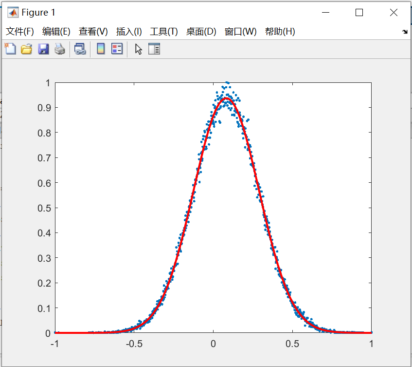
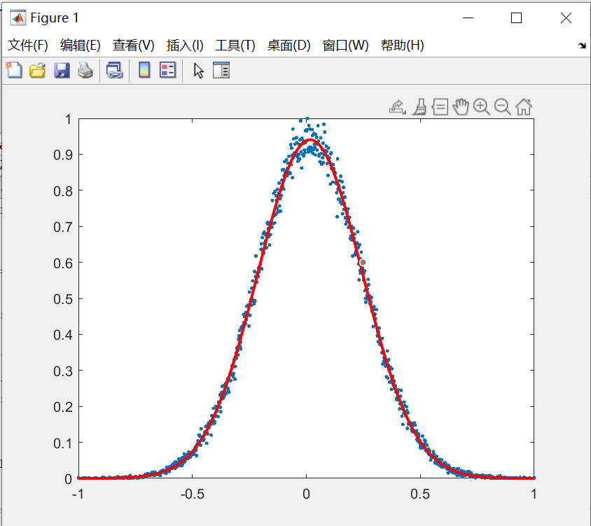
Finally, import the data in txt text into maltab for verification (g1 on the left and g2 on the right). The simulation results basically conform to the random number of Gaussian distribution