Thesis reading preparation

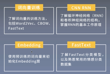
Preliminary knowledge reserve

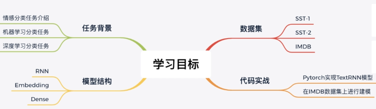
Learning objectives

Thesis Guide

Research background, achievements and significance of this paper

Research background

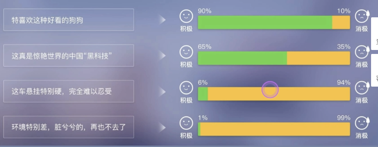
Application scenarios of emotion classification task: comment analysis, data mining analysis, public opinion analysis

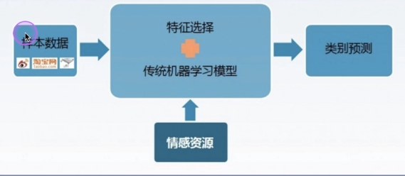
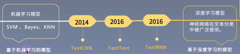
Emotion classification based on machine learning

Emotion classification based on deep learning
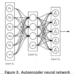
Feedforward neural network

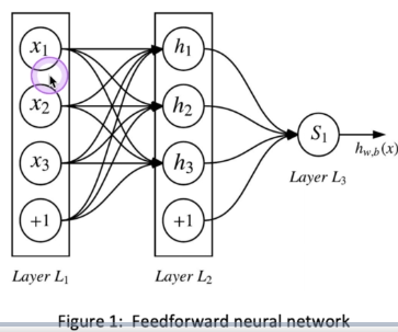
There is no need to define features manually, just learn the model by itself.

Autoencoder

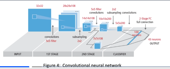
Convolutional neural network

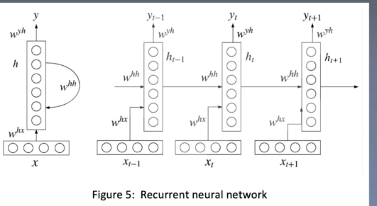
Cyclic neural network

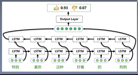
Combined structure of cyclic neural network

data set

research meaning

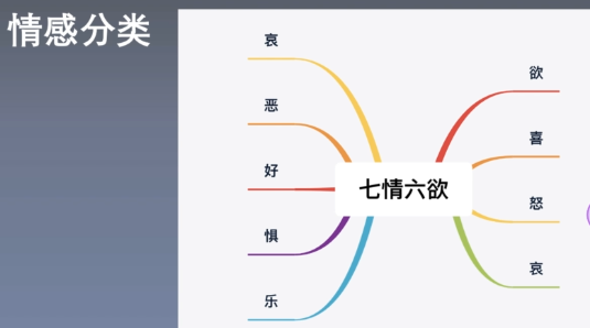
Emotional classification background

In the stage of machine learning model, some features need to be constructed manually.

Extensive reading of papers

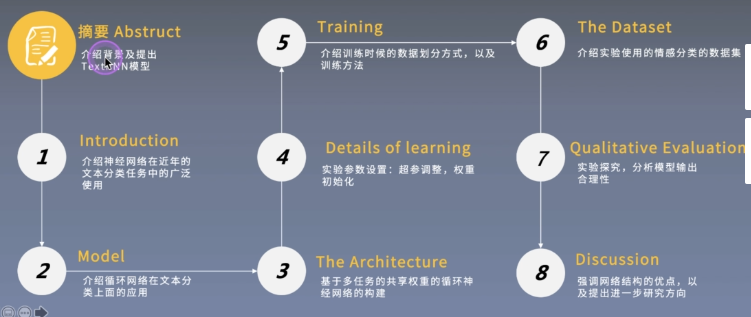
Thesis structure

abstract

Abstract core

• 1. In order to deal with the small amount of data, the commonly used method is to use an unsupervised pre training model, such as word vector. Good results have been achieved in the experiment, but such methods are indirect to improve the network effect;
• 2. Aiming at the text multi classification task, the author puts forward the method of multi task training and sharing model weight based on RNN, and puts forward three information sharing mechanisms;
• 3. The author models the text with specific tasks and achieves good results in the text classification task with four benchmarks.

Intensive reading of papers

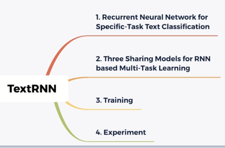
Overview of algorithm model in this paper

Knowledge tree

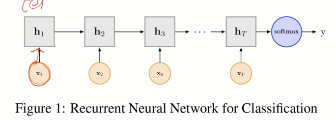
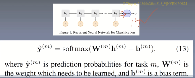
RNN structure

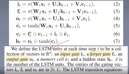
Variable length LSTM

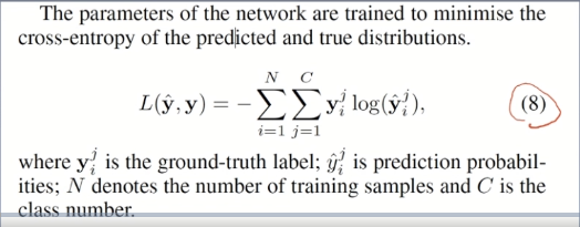
Definition of loss function

Details of algorithm model in this paper

Detail 1

Weight sharing
Neural network can solve many NLP tasks in multitasking learning. The author believes that multitasking learning can also be applied to emotion classification tasks. The author uses this shared representation of one to many words.

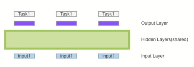
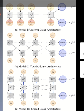
The tasks in the figure share the hidden layer in the middle. Since the input and output of different tasks may be different, the input layer and output layer cannot be shared. Based on this idea, the middle shared layer has many different methods, input and output, and puts forward three different structures:
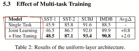
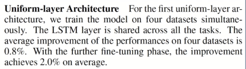
Uniform-Layer

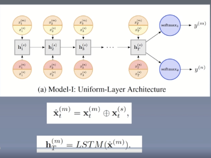
The middle part is shared. There are two inputs above and below. It inputs two tasks to calculate at the same time. When inputting, make corresponding softmax respectively. Further, we have four data sets, that is, there are four different tasks. Suppose task1 above and task2 below. The two tasks can be mixed for training. x(s)t represents the shared representation, x(m)t is a value to be input, and then add an x(s)t representation. The initial value of x(s)t is generated randomly, and then training is carried out continuously.
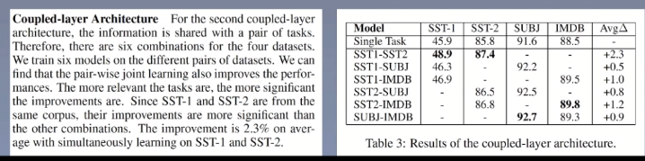
Coupled-Layer
Implemented using two lstms

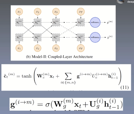
Each task has its own lstm layer. It is considered that there will not be too much impact between the two tasks and will focus more on its own tasks. The two tasks are carried out at the same time, and the outputs of the two tasks will be mixed, which can capture some information in other tasks.
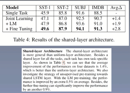
Shared-Layer

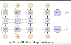
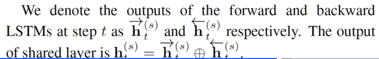
This model combines the advantages of the first two models. The shared weight is also in the middle. It is a two-way lstm. The main formula is as follows:

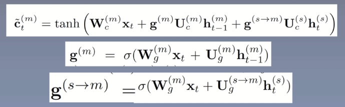
The information of the shared layer is mixed into the input, and h(s)t has the characteristics of two tasks.
Model comparison

• Uniform layer architecture: for each classification task, a randomly generated trainable vector is spelled after the embedding vector of each input character, indicating that all tasks share the LSTM layer in the specific task, and the hidden state at the last time is passed into softmax as an input. The shared parts of the model are: the randomly generated trainable vector in the input part and the shared LSTM layer;
• Coupled layer architecture: each task has its own independent LSTM layer, but the hidden state of all tasks at each time will be used as input together with the character of the next time, and the hidden state of the last time will be classified;
• Model 3 (shared layer architecture): in addition to a shared Bi lstm layer for obtaining shared information, each task has its own independent lstm layer, and the input of lstm includes the character of each time and the hidden state of Bi lstm.

Training process

train

loss

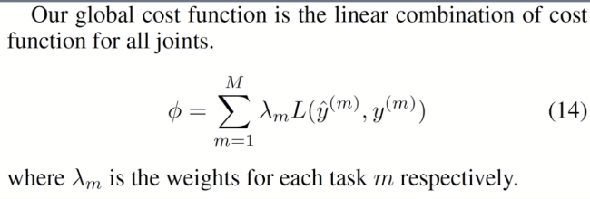
λ m consider the number of data sets, types of categories, etc.

Selection of data

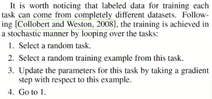
Training method:

• 1. Select a task at random;
• 2. Randomly select a training sample from the task;
• 3. Update the parameters according to the gradient based optimization (adagrad update rule is used in the paper);
• 4. Repeat steps 1 to 3.

Fine tuning

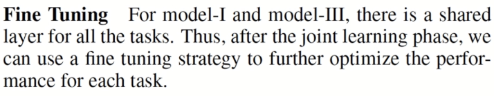
Pre training

Experimental setup and result analysis

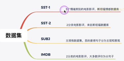
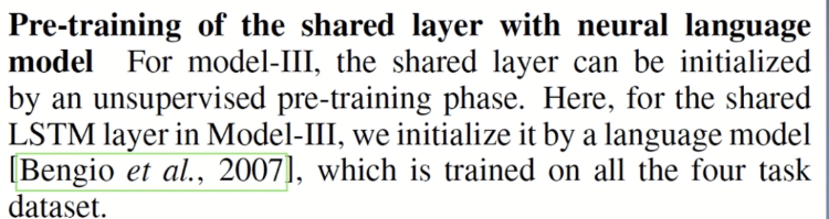
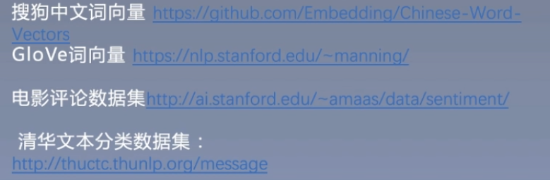
data set

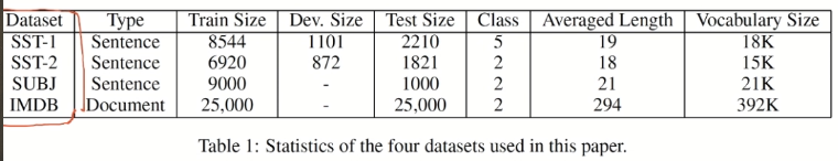
• Sst-1: movie reviews of five emotion categories, from Stanford emotion database
• Sst-2: 2 category film reviews, from Stanford database
• SUBJ: subjective data set. The purpose of the task is to divide sentences into subjective and objective
• IMDb: 2 categories of film reviews, most of which are long sentences

Analysis of super parameters

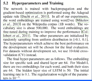
Use Word2vec to obtain word vectors in Wiki corpus, with a dictionary scale of about 500000. Word embedding is fine tuned during training to improve performance; Other parameters are sampled randomly in the range of [- 0.1,0.1], and the super parameter will select the group with the best performance in the verification set. For datasets without validation set, 10% off cross validation is used.
The embedding size of specific task and sharing layer is 64. For model 1, there are two embeddings for each word, both of which are 64. The hidden layer size of LSTM is 50. The initial learning rate was 0.1. The regularization weight of the parameter is 10-5.

experimental result

Model I

Model II

Model three

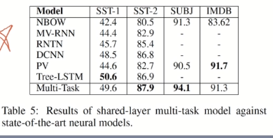
The above experiment is the internal comparison of the model. Let's take a look at the results compared with other models.

SOTA comparison

Visual analysis

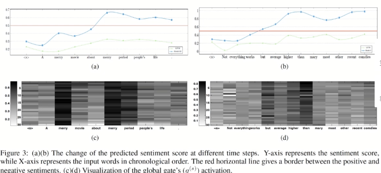
The author uses single-layer LSTM to compare with model 3. For the emotion classification of hidden state at each moment, the author intuitively shows the contribution of each word to the model.

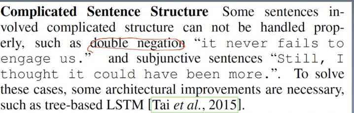
error analysis

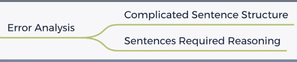
(1) Complex sentence structure (2) sentences in specific context

Paper summary

Key points

• Shared layer
• Multi task learning
• Pre training - pre training

Innovation points

• Shared weight
• Multi task hybrid training
• RNN structure for emotion data classification

Inspiration Point

• Multitasking training
  Multi-task Learning
• Multi task shared weight
  The differences among them are the mechanisms of sharing information among the several tasks.
• Performance improvement
  Experimental results show that our models can imporve the performances of a group of related tasks by exploring common features.
• Research on character level sharing mechanism
  In future work, we would like to investigate the other sharing mechanisms of the different task.

import torch
from torchtext import data

SEED = 1234

torch.manual_seed(SEED)
torch.backends.cudnn.deterministic = True

TEXT = data.Field(tokenize = 'spacy')
LABEL = data.LabelField(dtype = torch.float)
'''
Another handy feature of torchtext is that it has support for common datasets used in natural language processing.
The following code automatically downloads the IMDB dataset and splits it into the canonical train/test splits as torchtext.datasets objects. It process the data using the Fields we have previous defined. The IMDB dataset consists of 50,000 movie reviews, each marked as being a positive or negatice review.
'''
from torchtext import datasets
train_data,test_data = datasets.IMDB.splits(TEXT, LABEL)
# We can see how many examples are in each split by checking their length.
print(f'number of training examples:{len(train_data)}')
print(f'number of testing examples:{len(test_data)}')
# We can also check an example
print(vars(train_data.examples[0]))
'''
The IMDB dataset only has train/test splits, so we need to create a validation set. We can do this with the .split() method. By default this splits 70/30, however by passing a split_ratio argument, we can change the ratio argument, we can change the ratio of the split, i.e. a split_ratio of 0.8 would mean 80% of the examples make up the training set and 20% make up the validation set.
We also pass our random seed to the random_state argument, ensuring that we get the same train/validation split each time.
'''
import random
train_data, valid_data = train_data.split(random_state = random.seed(SEED))
# Again, we'll view how many examples are in each split.
print(f'Number of training examples:{len(train_data)}') #17500
print(f'Number of validing examples:{len(valid_data)}') #7500
print(f'Number of testing examples:{len(test_data)}') #25000

# The following builds the vocabulary, only keeping the most common max_size tokens.
MAX_VOCAB_SIZE = 25_000
TEXT.build_vocab(train_data, max_size=MAX_VOCAB_SIZE)
LABEL.build_vocab(train_data)

print(f'Unique tokens in TEXT vocabulary:{len(TEXT.vocab)}') #25002
print(f'Unique tokens in LABEL vocabulary:{len(LABEL.vocab)}') #2
# We can also view the most common words in the vocabulary and theri frequencies.
print(TEXT.vocab.freqs.most_common(20))
#We can also see the vocabulary directly using either the stoi(string to int) or itos(int to string) method.
print(TEXT.vocab.itos[:10])
#We can also check the labels, ensuring 0 is for negative and 1 is for positive.
print(LABEL.vocab.stoi)
'''
The final step of preparing the data is creating the iterators. We iterate over these in the training/evaluation loop, and they return a batch of examples(indexed and converted into tensors) at each iteration.
We'll use a BucketIterator which is a special type of iterator that will return a batch of examples where each example is of a similar length, minimizing the amount of padding per example.
We also want to place the tensors returned by the iterator on the GPU(if you're using one).PyTorch handles this using torch.device, we then pass this device to the iterator.
'''
BATCH_SIZE = 64
device = torch.device('cuda' if torch.cuda.is_available() else 'cpu')
train_iterator, valid_iterator,test_iterator = data.BucketIterator.splits(
	(train_data, valid_data, test_data),
	batch_size=BATCH_SIZE,
	device=device)

#model
import torch.nn as nn
class RNN(nn.Module):
	def __init__(self, input_dim, embedding_dim, hidden_dim, output_dim):
		super().__init__()
		self.embedding = nn.Embedding(input_dim, embedding_dim)
		self.rnn = nn.RNN(embedding_dim, hidden_dim)
		self.fc = nn.Linear(hidden_dim, output_dim)
	def forward(self, text):
		embedded = self.embedding(text) #text=[sent_len, batch_size]
		output, hidden = self.rnn(embedded)
		#output = [sent_len, batch_size, hid_dim]
		#hidden = [1, batch_size, hid_dim]
		assert torch.equal(output[-1,:,:],hidden.squeeze(0))
		return self.fc(hidden.squeeze(0))
'''
We now create an instance of our RNN class.
The input dimension is the dimension of the one-hot vectors.which is equal to the vocabulary size.
The embedding dimension is the size of the dense word vectors.This is usually around 50-250 dimensions, but depends on the size of the vocabulary.
The hidden dimension is the size of the hidden states.This is usually around 100-500 dimensions, but also depends on factors such as on the vocabulary size, the size of the dense vectors and compleity of the task.
The output dimension is usually the number of classes, however in the case of only 2 classes the output value is between 0 and 1 and thus can be 1-dimensional, i.e. a single scalar real number.
'''
INPUT_DIM = len(TEXT.vocab)
EMBEDDING_DIM = 100
HIDDEN_DIM = 256
OUTPUT_DIM = 1

model = RNN(INPUT_DIM EMBEDDING_DIM, HIDDEN_DIM, OUTPUT_DIM)
# Let's also create a function that will tell us how many trainable parameters our model has so we can compare the number of parameters across different models.
def count_parameters(model):
	return sum(p.unmel() for p in model.parameters() if p.requires_grad)
print(f'The model has {count_parameters(model):,}trainable parameters')

#create an optimizer
import torch.optim as optim
optimizer = optim.SGD(model.parameters(), lr=1e-3)
#define loss function
criterion = nn.BCEWithLogitsLoss()
# Using .to, we can place the model and the criterion on the GPU
model = model.to(device)
criterion = criterion.to(device)

def binary_accuracy(pred, y):
	'''
	Return accuracy per batch, i.e. if you get 8/10 right, this returns 0.8,Not 8
	'''
	# round predictions to the closest integer
	rounded_preds = torch.round(torch.sigmoid(preds))
	correct = (rounded_preds == y).float()#convert into float for division
	acc = correct.sum() / len(correct)
	return acc

def train(model, iterator, optimizer, criterion):
	epoch_loss = 0
	epoch_acc = 0
	model.train()
	for batch in iterator:
		optimizer.zero_grad()
		predictions = model(batch.text).squeeze(1)
		loss = criterion(predictions, batch.label)
		loss.backward()
		optimizer.step()
		epoch_loss +=  loss.item()
		epoch_acc +=acc.item()
	return epoch_loss/len(iterator), epoch_acc/len(iterator)
def evaluate(model, iterator, criterion):
	epoch_loss = 0
	epoch_acc = 0
	model.eval()
	with torch.no_grad():
		for batch in iterator:
			predictions = model(batch.text).squeeze(1)
			loss = criterion(predictions, batch.label)
			acc = binary_accuracy(predictions, batch.label)
			epoch_loss += loss.item()
			epoch_acc += acc.item()
	return epoch_loss/len(iterator), epoch_acc/len(iterator)
import time
def epoch_time(start_time, end_time):
	elapsed_time = end_time-start_time
	elapsed_mins = int(elapsed_time / 60)
	elapsed_secs = int(elapsed_time - (elapsed_mins*60))	
	return elapsed_mins, elapsed_secs
'''
We then train the model through multiple ephchs, an epoch being a complete pass through all examples in the training and validation sets.
At each epoch, if the validation loss is the best we have seen so far, we'll save the parameters of the model and then after training has finished we'll use that model on the test set.
'''
N_EPOCH = 5
best_valid_loss = float('inf')
for epoch in range(N_EPOCH):
	start_time = time.time()
	train_loss, train_acc = train(model, train_iterator, optimizer, criterion)
	valid_loss, valid_acc = evaluate(model, valid_iterator, criterion)
	end_time = time.time()
	epoch_mins, epoch_secs = epoch_time(start_time, end_time)
	if valid_loss<best_valid_loss:
		best_valid_loss = valid_loss
		torch.save(model.state_dict(),'tuti-model.pt')
	print(f'Epoch:{epoch+1:02} | Epoch Time:{epoch_mins}m {epoch_secs}s')
	print(f'\tTrain Loss:{train_loss:.3f} | Train Acc:{train_acc*100:.2f}%')
	print(f'\tVal Loss:{valid_loss:.3f} | Val Acc:{valid_acc*100:.2f}%')
'''
You may have noticed the loss is not really decreasing and the accuracy is poor. This is due to several issues with the model which we'll imporve int the next notebook.
Finally,the metric we actually care about,the test loss and accuracy,which we get from our parameters that gave us the best validation loss.
'''
model.load_state_dict(torch.load('tuti-model.pt'))
test_loss, test_acc = evaluate(model, test_iterator, criterion)
print(f'Test Loss:{test_loss:.3f} | Test acc:{test_acc*100}:.2f%')