Reinforcement learning - from Q-Learning to DQN(Deep Q-Network)

Reinforcement learning is a kind of learning that maps from environment state to action. The goal is to maximize the cumulative reward in the process of agent interaction with environment.
This process can be explained as that at time t, the agent agent makes an action based on the state of the current environment. Then, after the action acts on the state of the current environment, it returns a reward to the agent agent, and then the agent enters the state of time t+1.

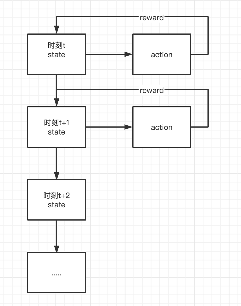
agent, environment, reward and action can abstract the problem into a Markov decision process.

Q-Learning

Q-Learning is a classical algorithm in reinforcement learning. It mainly relies on the Q table to store State and Action, and selects the Action with the maximum benefit according to the Q value.
Table Q is used to record the values of status action pairs. The initialization format is shown in the table below.

	action1	action2	action3	...
state1	q(state1, action1)	q(state1, action2)	q(state1, action3)
state2	q(state2, action1)	q(state2, action2)	q(state2, action3)
state3	q(state3, action1)	q(state3, action2)	q(state3, action3)
...

The update formula of table Q is as follows, where α \alpha α For learning rate, γ \gamma γ Is the reward decay coefficient, and r is the reward of action a
Q ( s , a ) ← Q ( s , a ) + α [ r + γ m a x a ′ Q ( s ′ , a ′ ) − Q ( s , a ) ] . Q(s,a) \gets Q(s,a) + \alpha[r + \gamma max_{a'}Q(s', a') - Q(s,a)]. Q(s,a)←Q(s,a)+α[r+γmaxa′​Q(s′,a′)−Q(s,a)].
According to Q(s,a) in the past Q table as Q estimation, select the largest Q (s', a ') in the next state s' and multiply it by the decay coefficient γ \gamma γ Add the real return value as Q reality.
In order to verify the update process of Q-Learning, an example of a well-known boss is cited.
Zhihu link

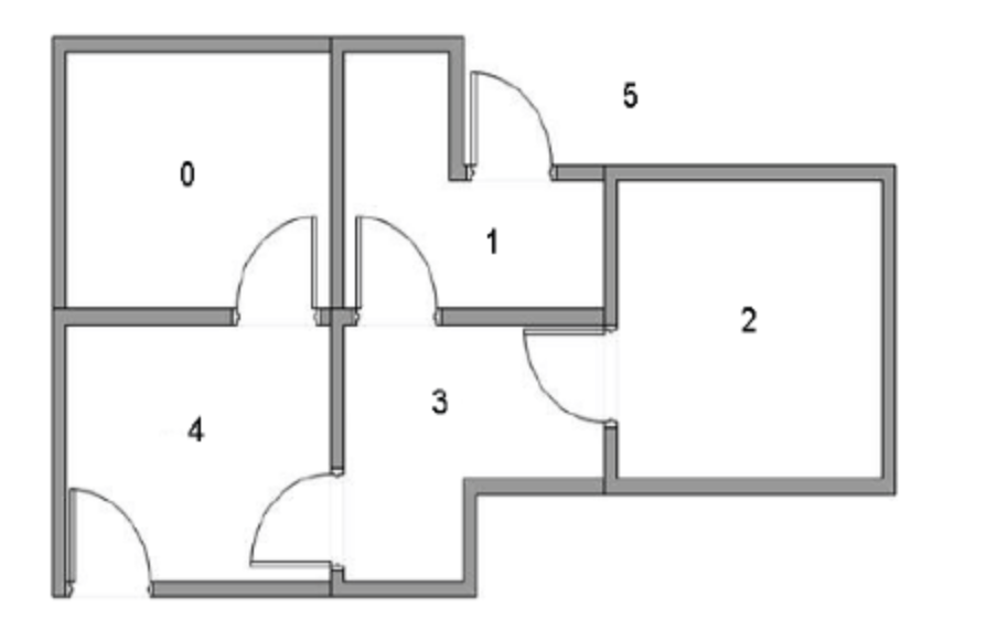
There is a 5-room house, as shown in the figure below. Rooms are connected through doors. Numbers 0 to 4 and 5 are outside the house, that is, our destination. We randomly place the agent in any room and return a reward every time we open a door.

The following figure shows the abstract relationship between rooms. The arrow indicates that the agent can transfer from the room to the connected room, and the number on the arrow represents the reward value.

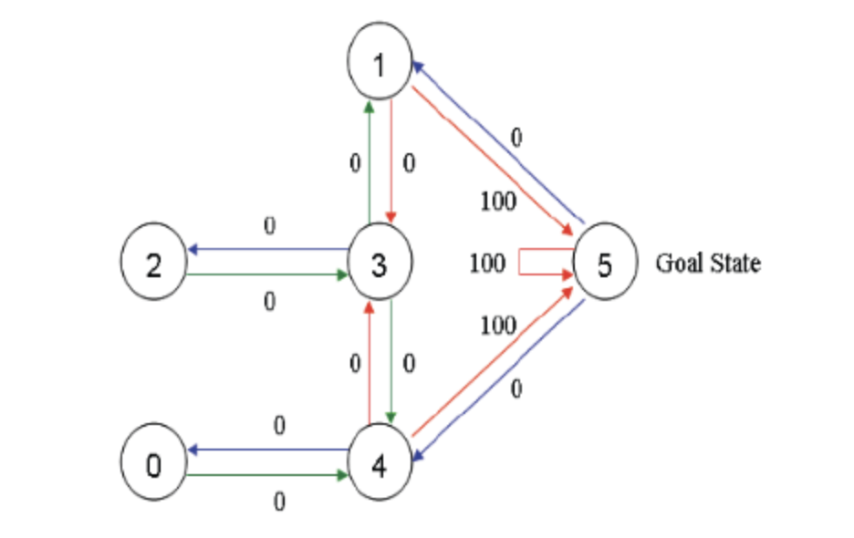
Therefore, the following return matrix can be obtained

   [[-1,-1,-1,-1,0,-1],
   [-1,-1,-1,0,-1,100],
   [-1,-1,-1,0,-1,-1],
   [-1,0, 0, -1,0,-1],
   [0,-1,-1,0,-1,100],
   [-1,0,-1,-1,0,100]]

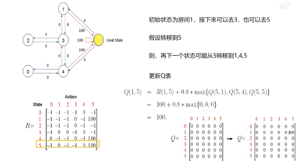
Set learning rate α \alpha α= 1. Reward decay coefficient γ \gamma γ It is 0.8, and the update process is shown in the figure below.

python code

import numpy as np
GAMMA = 0.8
Q = np.zeros((6, 6))
# Initial matrix
R=np.asarray(
   [[-1,-1,-1,-1,0,-1],
   [-1,-1,-1,0,-1,100],
   [-1,-1,-1,0,-1,-1],
   [-1,0, 0, -1,0,-1],
   [0,-1,-1,0,-1,100],
   [-1,0,-1,-1,0,100]]
)

def getMaxQ(state):
    return max(Q[state, :])
def QLearning(state):
    curAction = None
    for action in range(6):
        if(R[state][action] == -1):
            Q[state, action] = 0
        else:
            curAction = action
            Q[state, action] = R[state][action] + GAMMA * getMaxQ(curAction)
count=0
while count < 1000:
    for i in range(6):
        QLearning(i)
    count += 1
print(Q)

The final Q table matrix is

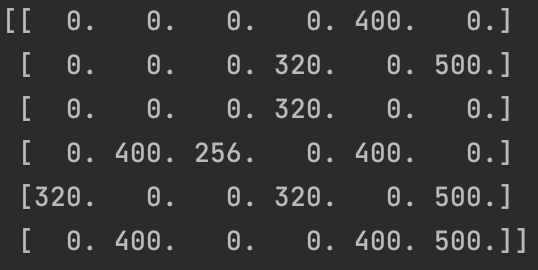
Why is the maximum value of Q table matrix 500?
This is because we set the learning rate α \alpha α= 1. Reward decay coefficient γ \gamma γ For the reason of 0.8, when we select state = 5 and action = 5, that is, when updating Q [5,5], Q [5,5] = R [5] [5] + 0.8 * max{Q [5,1], Q [5,4], Q [5,5]} = 500, so the maximum value in the Q table can only be 500.
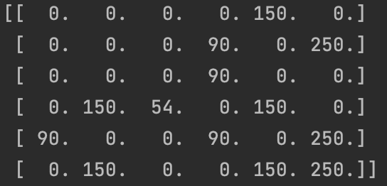
When we put the reward decay coefficient γ \gamma γ Change to 0.6 to get the final Q-table matrix as

Q-Learning method can solve the problem of small state space and action space. For the problem of huge state space and action space, the memory overhead of creating a Q table is very large. In addition, the limitation of data volume and time overhead is also a defect of Q-Learning algorithm.

DQN(Deep Q-Network)

DQN (Deep Q-Network) is a revolutionary algorithm that combines deep learning and reinforcement learning to realize end-to-end from perception to action. When our Q table is too large to be established, using DQN is a good choice.

Before introducing DQN(Deep Q-Network), learn about the Function Approximation method.
The value function approximation method is to solve the problem of too large state space, also known as "dimensional disaster". It can also be regarded as a fitting function to store the state and action by replacing the Q table with a nonlinear or linear function ω \omega ω The process of weighting.
v ^ ( s , ω ) ≈ v π ( s ) o r q ^ ( s , a , ω ) ≈ q π ( s , a ) \hat{v}(s, \omega) \approx v_\pi(s) or \hat{q}(s, a, \omega) \approx q_\pi(s,a) v^(s,ω)≈vπ​(s)orq^​(s,a,ω)≈qπ​(s,a)

As a deep reinforcement learning model, DQN combines the convolutional neural network with the Q-Learning algorithm in traditional reinforcement learning, turns the Q table of Q-Learning into Q-Network, takes the input state extraction feature as the input, calculates the value function through MC/TD as the output, and then trains the function parameter w weight until the model converges.

Training samples are collected mainly through ε − g r e e d y \varepsilon-greedy ε − green strategy generation. Generally, the first few episodes are used to generate samples, and the later episodes are used for model training. That is, the batch processing method is used to save some samples first, and then take some samples from them to update the Q network. This method is also called experience playback. This method can solve the problem of strengthening the relevance of learning collected samples and break the correlation between data, so as to improve the stability of the algorithm.
The loss function of the model is calculated by the mean square deviation of the real Q value and the simulated Q value.

q π ( s , a ) = r + γ m a x a ′ q ( s ′ , a ′ , ω ) q_\pi(s, a) = r+\gamma max_{a'}q(s',a',\omega) qπ​(s,a)=r+ γ maxa′​q(s′,a′, ω) S' is the next time state
J ( ω ) = E π [ ( q π ( s , a ) − q ^ ( s , a , ω ) ) 2 ] J(\omega) = E_\pi[(q_\pi(s, a) - \hat{q}(s,a,\omega))^2] J(ω)=Eπ​[(qπ​(s,a)−q^​(s,a,ω))2]

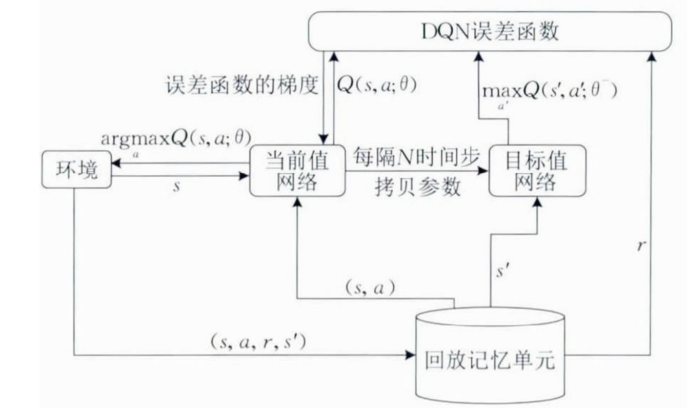
The DQN training process is shown in the figure below

python code

"""
Dependencies:
torch: 0.4
gym: 0.8.1
numpy
"""
import torch
import torch.nn as nn
import torch.nn.functional as F
import numpy as np
import gym
import pickle

# Hyper Parameters
BATCH_SIZE = 32
LR = 0.01                   # learning rate
EPSILON = 0.9               # greedy policy
GAMMA = 0.9                 # reward discount
TARGET_REPLACE_ITER = 100   # target update frequency
# Number of memory lines
MEMORY_CAPACITY = 2000
# Introducing the CartPole environment of gym
env = gym.make('CartPole-v0')
env = env.unwrapped

# Get status
# 2
N_ACTIONS = env.action_space.n
# 4
N_STATES = env.observation_space.shape[0]
ENV_A_SHAPE = 0 if isinstance(env.action_space.sample(), int) else env.action_space.sample().shape     # to confirm the shape



# neural network
class Net(nn.Module):
    def __init__(self, ):
        super(Net, self).__init__()
        # Enter observations
        self.fc1 = nn.Linear(N_STATES, 50)
        # Using quadratic distribution to generate initial weights
        self.fc1.weight.data.normal_(0, 0.1)   # initialization
        # Output the value of each action
        self.out = nn.Linear(50, N_ACTIONS)
        self.out.weight.data.normal_(0, 0.1)   # initialization

    def forward(self, x):
        x = self.fc1(x)
        x = F.relu(x)
        # Returns the value of each action
        actions_value = self.out(x)
        return actions_value

# DQN network
class DQN(object):
    def __init__(self):
        # For the same network with different parameters, the parameters of eval are updated every time, which is always several versions faster than the target
        self.eval_net, self.target_net = Net(), Net()
        # Record how many steps you have learned
        self.learn_step_counter = 0                                     # for target updating
        # Memory location
        self.memory_counter = 0                                         # for storing memory
        # Initialize memory s, a, r, s_
        self.memory = np.zeros((MEMORY_CAPACITY, N_STATES * 2 + 2))     # initialize memory
        self.optimizer = torch.optim.Adam(self.eval_net.parameters(), lr=LR)
        self.loss_func = nn.MSELoss()
    # Take action
    def choose_action(self, x):
        x = torch.unsqueeze(torch.FloatTensor(x), 0)
        # input only one sample
        # Random selection probability
        if np.random.uniform() < EPSILON:   # greedy selects the action with the greatest value
            actions_value = self.eval_net.forward(x)
            action = torch.max(actions_value, 1)[1].data.numpy()
            action = action[0] if ENV_A_SHAPE == 0 else action.reshape(ENV_A_SHAPE)  # return the argmax index
        else:   # random
            action = np.random.randint(0, N_ACTIONS)
            action = action if ENV_A_SHAPE == 0 else action.reshape(ENV_A_SHAPE)
        return action
    # Memory storage
    def store_transition(self, s, a, r, s_):
        transition = np.hstack((s, [a, r], s_))
        # replace the old memory with new memory
        # If the memory is full, cover the old memory
        index = self.memory_counter % MEMORY_CAPACITY
        self.memory[index, :] = transition
        self.memory_counter += 1
    # Extract learning from memory
    def learn(self):
        # target parameter update
        # Every 100 learn_step_counter to update the target_net
        if self.learn_step_counter % TARGET_REPLACE_ITER == 0:
            self.target_net.load_state_dict(self.eval_net.state_dict())
        self.learn_step_counter += 1

        # sample batch transitions
        # Random extraction memory
        sample_index = np.random.choice(MEMORY_CAPACITY, BATCH_SIZE)
        # Take out all the items corresponding to the memory
        b_memory = self.memory[sample_index, :]
        b_s = torch.FloatTensor(b_memory[:, :N_STATES])
        b_a = torch.LongTensor(b_memory[:, N_STATES:N_STATES+1].astype(int))
        b_r = torch.FloatTensor(b_memory[:, N_STATES+1:N_STATES+2])
        b_s_ = torch.FloatTensor(b_memory[:, -N_STATES:])

        # q_eval w.r.t the action in experience
        # Select the current state and apply the value of the action
        q_eval = self.eval_net(b_s).gather(1, b_a)  # shape (batch, 1)
        # The value of the next status, plus detach, makes the target network not updated, because the target parameter is through target_ REPLACE_ Updated by ITER
        q_next = self.target_net(b_s_).detach()     # detach from graph, don't backpropagate
        # Calculate the target value using the current action reward and future status
        q_target = b_r + GAMMA * q_next.max(1)[0].view(BATCH_SIZE, 1)   # shape (batch, 1)
        # Calculate the difference between the real value and the estimated value
        loss = self.loss_func(q_eval, q_target)

        self.optimizer.zero_grad()
        loss.backward()
        self.optimizer.step()

dqn = DQN()
print('\nCollecting experience...')

ep_r_list = []
for i_episode in range(400):
    # Get a feedback based on your current environment
    s = env.reset()
    # print("state", s)
    ep_r = 0
    while True:
        # Environment Rendering
        env.render()
        # Select action 0 or 1 according to the state and swing left and right
        a = dqn.choose_action(s)
        # print("action", a)
        # take action
        # Feedback from environmental actions s_ The next status r returns whether done ends this round of info. I don't know what to do
        s_, r, done, info = env.step(a)
        # print("s_", s_)
        # print("r", r)
        # print("done", done)
        # print("info", info)

        # Calculate rewards
        # modify the reward
        x, x_dot, theta, theta_dot = s_
        # The straighter the pole, the better
        r1 = (env.x_threshold - abs(x)) / env.x_threshold - 0.8
        # It means that the position of the trolley closer to the middle is better
        r2 = (env.theta_threshold_radians - abs(theta)) / env.theta_threshold_radians - 0.5
        r = r1 + r2

        # print("r", r)
        # Storage feedback
        dqn.store_transition(s, a, r, s_)
        ep_r += r
        # If it's full
        if dqn.memory_counter > MEMORY_CAPACITY:
            dqn.learn()
            if done:
                print('Ep: ', i_episode,
                      '| Ep_r: ', round(ep_r, 2))
                ep_r_list.append((i_episode, round(ep_r, 2)))
        if done:
            break
        # The current state changes to the next state
        s = s_

with open('ep_r.pkl', 'wb') as f:
    pickle.dump(ep_r_list, f)

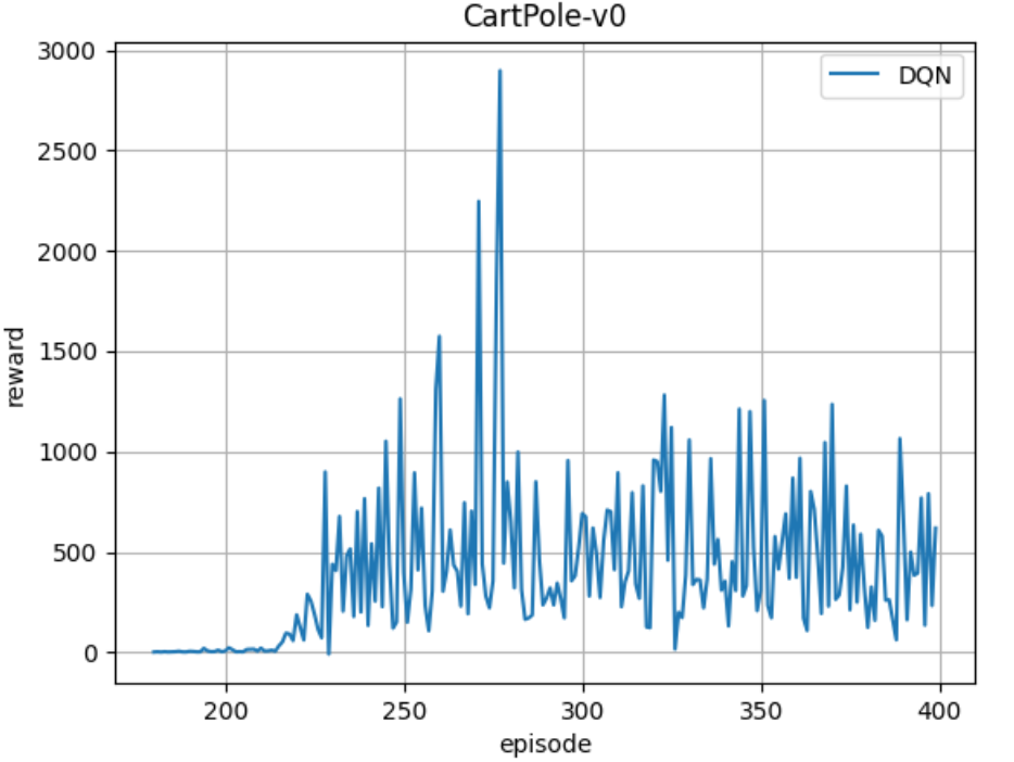
The average score is used as the evaluation index. When testing performance, the agent executes in a certain number of steps, records all reward values obtained by the agent and averages them.

Refer to the following blogs and tutorials

https://zhuanlan.zhihu.com/p/35882937
https://blog.csdn.net/qq_30615903/article/details/80744083
https://www.bilibili.com/video/BV1Vx411j7kT?p=27