preface

Numpy (short for numerical Python) is a library specially used for scientific calculation, which is mainly used for the processing of multidimensional arrays (matrices).

Because the bottom layer of Numpy is developed in C language, it is much faster than the list of native Python when dealing with some multi-dimensional arrays (matrices).

Numpy is a basic scientific computing library, and most of Python's other scientific computing extensions are based on it.

Installation:

Enter your own environment, and then enter conda install numpy to install. After installation, if the following errors occur when using pycharm in the future:

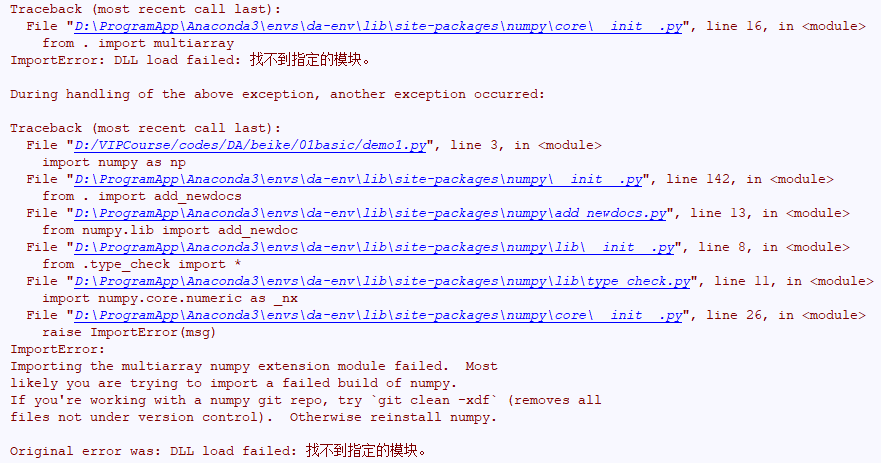
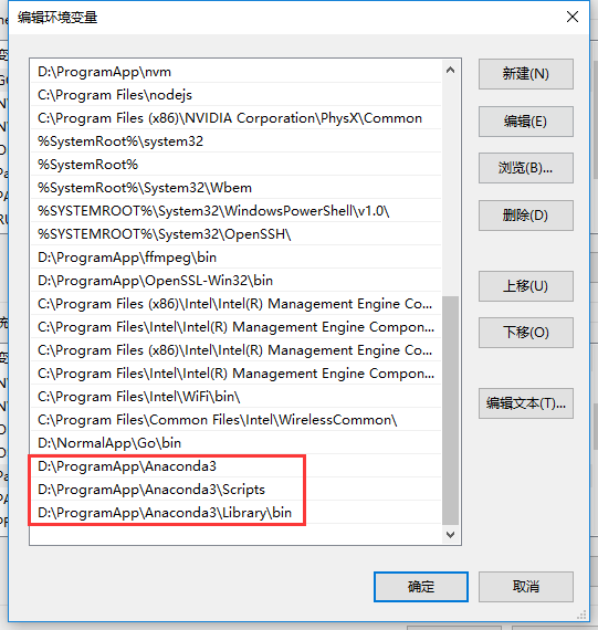
Then you need to add the installation PATH of Anaconda to the environment variable of PATH. For example, if I install Anaconda in D:\ProgramApp\Anaconda, I need to add the following three environment variables:

Introduction to Numpy Library

NumPy is a powerful Python library, which is mainly used to perform calculations on multidimensional arrays.

The word NumPy comes from two words -- Numerical and Python. NumPy provides a large number of library functions and operations to help programmers easily perform Numerical calculations. It is widely used in the field of data analysis and machine learning. He has the following characteristics:

1. Numpy has built-in parallel computing function. When the system has multiple cores, numpy will automatically perform parallel computing when doing some computing.
2. The bottom layer of Numpy is written in C language, and the GIL (global interpreter lock) is released internally. Its operation speed on the array is not limited by the Python interpreter, and its efficiency is much higher than that of pure Python code.
3. There is a powerful N-dimensional Array object Array (something similar to a list).
4. Practical linear algebra, Fourier transform and random number generation function.

In short, it is a very efficient package for dealing with numerical operations.

Installation:

You can install numpy via PIP install.

Tutorial address:

1. Official website: https://docs.scipy.org/doc/numpy/user/quickstart.html .
2. Chinese documents: https://www.numpy.org.cn/user_guide/quickstart_tutorial/index.html.

Performance comparison between Numpy array and Python list:

For example, we want to square each element in a Numpy array and Python list. Then the code is as follows:

# How Python lists
t1 = time.time()
a = []
for x in range(100000):
    a.append(x**2)
t2 = time.time()
t = t2 - t1
print(t)

The time spent is about 0.07180. If you use numpy array, the speed will be much faster:

t3 = time.time()
b = np.arange(100000)**2
t4 = time.time()
print(t4-t3)

Basic usage of NumPy array

1. Numpy is a Python scientific computing library used to quickly process arrays of arbitrary dimensions.
2. NumPy provides an N-dimensional array type ndarray, which describes a collection of "items" of the same type.
3. numpy.ndarray supports vectorization.
4. NumPy is written in c language, and the GIL is released at the bottom. Its operation speed on the array is no longer limited by the python interpreter.

Array in numpy:

The use of arrays in Numpy is very similar to lists in Python. The differences between them are as follows:

1. Multiple data types can be stored in a list. For example, a = [1,'a'] is allowed, while arrays can only store the same data type.
2. Arrays can be multidimensional. When all the data in multidimensional arrays are numerical types, they are equivalent to matrices in linear algebra and can operate on each other.

Create an array (np.ndarray object):

Numpy often deals with arrays, so the first step is to learn to create arrays. The data type of the array in numpy is called ndarray. Here are two ways to create:

1. Generated from lists in Python:

   import numpy as np
   a1 = np.array([1,2,3,4])
   print(a1)
   print(type(a1))
   

2. It is generated using np.arena. The usage of np.arena is similar to range in Python:

   import numpy as np
   a2 = np.arange(2,21,2)
   print(a2)
   

3. Use np.random to generate an array of random numbers:

   a1 = np.random.random(2,2) # Generates an array of random numbers with 2 rows and 2 columns
   a2 = np.random.randint(0,10,size=(3,3)) # The element is a random array of 3 rows and 3 columns from 0 to 10
   

4. Use the function to generate a special array:

   import numpy as np
   a1 = np.zeros((2,2)) #Generate an array of 2 rows and 2 columns with all elements of 0
   a2 = np.ones((3,2)) #Generate an array of 3 rows and 2 columns with all elements being 1
   a3 = np.full((2,2),8) #Generate an array of 2 rows and 2 columns with all elements of 8
   a4 = np.eye(3) #Generate a 3x3 matrix with element 1 and other elements 0 on the skew square
   

Common properties of ndarray:

ndarray.dtype:

Because the array can only store the same data type, you can get the data type of the elements in the array through dtype. The following are the common data types of ndarray.dtype:

data type	describe	Unique identifier
bool	Boolean type (True or False) stored in one byte	'b'
int8	One byte size, - 128 to 127	'i1'
int16	Integer, 16 bit integer (- 32768 ~ 32767)	'i2'
int32	Integer, 32-bit integer (- 2147483648 ~ 2147483647)	'i4'
int64	Integer, 64 bit integer (- 9223372036854775808 ~ 9223372036854775807)	'i8'
uint8	Unsigned integer, 0 to 255	'u1'
uint16	Unsigned integer, 0 to 65535	'u2'
uint32	Unsigned integer, 0 to 2 * * 32 - 1	'u4'
uint64	Unsigned integer, 0 to 2 * * 64 - 1	'u8'
float16	Semi precision floating point number: 16 bits, sign 1 bit, index 5 bits, precision 10 bits	'f2'
float32	Single precision floating point number: 32 bits, sign 1 bit, exponent 8 bits, precision 23 bits	'f4'
float64	Double precision floating point number: 64 bits, sign 1 bit, index 11 bits, precision 52 bits	'f8'
complex64	Complex number, which represents the real part and imaginary part with two 32-bit floating-point numbers respectively	'c8'
complex128	Complex numbers, representing the real part and imaginary part with two 64 bit floating-point numbers respectively	'c16'
object_	python object	'O'
string_	character string	'S'
unicode_	unicode type	'U'

We can see that Numpy has many more types of values than Python's built-in, because Numpy is designed to efficiently process massive data. For example, if we want to store tens of billions of numbers, and these numbers are no more than 254 (within one byte), we can set dtype to int8, which can save memory space more than using int64 by default. Type related operations are as follows:

1. Default data type:

   import numpy as np
   a1 = np.array([1,2,3])
   print(a1.dtype) 
   # If it is a windows system, the default is int32
   # If it is a mac or linux system, it is determined according to the system
   

2. Specify dtype:

   import numpy as np
   a1 = np.array([1,2,3],dtype=np.int64)
   # Or a1 = np.array([1,2,3],dtype="i8")
   print(a1.dtype)
   

3. Modify dtype:

   import numpy as np
   a1 = np.array([1,2,3])
   print(a1.dtype) # In the window system, the default is int32
   # Modify dtype below
   a2 = a1.astype(np.int64) # astype does not modify the array itself, but returns the modified result
   print(a2.dtype)
   

ndarray.size:

Gets the total number of elements in the array. For example, there is a two-dimensional array:

   import numpy as np
   a1 = np.array([[1,2,3],[4,5,6]])
   print(a1.size) #6 is printed because there are a total of 6 elements

ndarray.ndim:

The dimension of the array. For example:

   a1 = np.array([1,2,3])   print(a1.ndim) # Dimension is 1   a2 = np.array([[1,2,3],[4,5,6]])   print(a2.ndim) # Dimension is 2   a3 = np.array([[[1,2,3],[4,5,6]],[[7,8,9],[10,11,12]]])   print(a3.ndim) # Dimension is 3

ndarray.shape:

The tuple of the dimension of the array. For example, the following code:

   a1 = np.array([1,2,3])   print(a1.shape) # output(3,)，It means a one-dimensional array with three data   a2 = np.array([[1,2,3],[4,5,6]])   print(a2.shape) # output(2,3)，It means a two bit array, 2 rows and 3 columns   a3 = np.array([       [           [1,2,3],           [4,5,6]       ],       [           [7,8,9],           [10,11,12]       ]   ])   print(a3.shape) # output(2,2,3)，It means a three-dimensional array. There are two elements in total. Each element is two rows and three columns   a44 = np.array([1,2,3],[4,5])   print(a4.shape) # output(2,)，intend a4 Is a one-dimensional array with a total of 2 columns   print(a4) # Output [list([1, 2, 3]) list([4, 5]), where the outermost layer is an array and the inner layer is a Python list

In addition, we can also modify the dimension of the array through ndarray.reshape. The example code is as follows:

   a1 = np.arange(12) #Generate a one-dimensional array with 12 data   print(a1)    a2 = a1.reshape((3,4)) #It becomes a two-dimensional array with 3 rows and 4 columns   print(a2)   a3 = a1.reshape((2,3,2)) #Into a three-dimensional array, a total of 2 blocks, each block is 2 rows and 2 columns   print(a3)   a4 = a2.reshape((12,)) # take a2 The two-dimensional array becomes a 12 column one-dimensional array   print(a4)   a5 = a2.flatten() # No matter how many dimensions a2 is, it will become a one-dimensional array print(a5)

Note that reshape does not modify the original array itself, but returns the modified result. If you want to modify the array itself directly, you can use resize instead of reshape.

ndarray.itemsize:

The size of each element in the array, in bytes. For example, the following code:

   a1 = np.array([1,2,3],dtype=np.int32)   print(a1.itemsize) # Print 4, because each byte is 8 bits, 32 bits / 8 = 4 bytes

Numpy array operation

Array broadcast mechanism:

Calculation of arrays and numbers:

In the Python list, if you want to add a number to all the elements in the list, you can either use the map function or loop the whole list. However, the array in NumPy can be operated directly on the array.

The example code is as follows:

import numpy as np
a1 = np.random.random((3,4))
print(a1)
# If you want to multiply all elements on the a1 array by 10, you can do so by
a2 = a1*10
print(a2)
# You can also use round to keep only 2 decimal places for all elements
a3 = a2.round(2)

The above example is multiplication. In fact, addition, subtraction and division are similar.

Array and array calculation:

1. Operations between arrays with the same structure:

   a1 = np.arange(0,24).reshape((3,8))
   a2 = np.random.randint(1,10,size=(3,8))
   a3 = a1 + a2 #Subtraction / division / multiplication are all possible
   print(a1)
   print(a2)
   print(a3)
   

2. Operations between arrays with the same number of rows and only 1 column:

   a1 = np.random.randint(10,20,size=(3,8)) #3 rows and 8 columns
   a2 = np.random.randint(1,10,size=(3,1)) #3 rows and 1 column
   a3 = a1 - a2 #The number of rows is the same, and a2 has only one column, which can operate on each other
   print(a3)
   

3. Operations between arrays with the same number of columns and only 1 row:

   a1 = np.random.randint(10,20,size=(3,8)) #3 rows and 8 columns
   a2 = np.random.randint(1,10,size=(1,8))
   a3 = a1 - a2
   print(a3)
   

Broadcasting principle:

If the axis lengths of the trailing dimension (i.e. the dimension from the end) of the two arrays match, or the length of one of them is 1, they are considered broadcast compatible. The broadcast will be on the missing and / or length 1 dimension.

Look at the following case analysis:

1. Can an array with shape of (3,8,2) operate with an array of (8,3)?
   Analysis: No, because according to the broadcasting principle, 2 and 3 in (3,8,2) and (8,3) are not equal from the back to the front, so the operation cannot be carried out.

2. Can an array with shape of (3,8,2) operate with an array of (8,1)?
   Analysis: Yes, because according to the broadcasting principle, although 2 and 1 in (3,8,2) and (8,1) are not equal, one side can participate in the operation because its length is 1.

3. Can an array with shape of (3,1,8) operate with an array of (8,1)?
   Analysis: Yes, because according to the broadcasting principle, 4 and 1 in (3,1,4) and (8,1) are not equal and 1 and 8 are not equal, but one of the two terms has a length of 1, so it can participate in the operation.

Operation of array shape:

Through some functions, it is very convenient to operate the shape of the array.

reshape and resize methods:

Both methods are used to modify the shape of the array, but there are some differences.

1. reshape is to convert the array into a specified shape, and then return the converted result. The shape of the original array will not change. Call method:

   a1 = np.random.randint(0,10,size=(3,4))
   a2 = a1.reshape((2,6)) #Return the modified result without affecting the original array itself
   

2. resize is to convert the array into a specified shape, which will directly modify the array itself. No value is returned. Call method:

   a1 = np.random.randint(0,10,size=(3,4))
   a1.resize((2,6)) #a1 itself has changed
   

flatten and t ravel methods:

Both methods convert multi-dimensional arrays into one-dimensional arrays, but there are the following differences:

1. flatten converts the array into a one-dimensional array and then returns the copy back, so subsequent modifications to the return value will not affect the previous array.
2. T ravel returns the view (which can be understood as a reference) after converting the array into a one-dimensional array, so subsequent modifications to the return value will affect the previous array.
   For example, the following code:

x = np.array([[1, 2], [3, 4]])
x.flatten()[1] = 100 #At this time, the position element of x[0] is still 1
x.ravel()[1] = 100 #At this time, the position element of x[0] is 100

Combination of different arrays:

If you want to combine multiple arrays, you can also use some of these functions.

1. vstack: stack arrays vertically. The array must have the same number of columns to stack. The example code is as follows:

   a1 = np.random.randint(0,10,size=(3,5))
   a2 = np.random.randint(0,10,size=(1,5))
   a3 = np.vstack([a1,a2])
   

2. Hsstack: stack arrays horizontally. The rows of the array must be the same to overlay. The example code is as follows:

   a1 = np.random.randint(0,10,size=(3,2))
   a2 = np.random.randint(0,10,size=(3,1))a3 = np.hstack([a1,a2])
   

3. concatenate([],axis): stack two arrays, but in the horizontal or vertical direction. It depends on the parameters of axis. If axis=0, it means stacking in the vertical direction (row). If axis=1, it means stacking in the horizontal direction (column). If axis=None, the two arrays will be combined into a one-dimensional array.
   It should be noted that if you stack horizontally, the rows must be the same, and if you stack vertically, the columns must be the same.

The example code is as follows:

a = np.array([[1, 2], [3, 4]])
b = np.array([[5, 6]])
np.concatenate((a, b), axis=0)
# result:
array([[1, 2],
    [3, 4],
    [5, 6]])

np.concatenate((a, b.T), axis=1)
# result:
array([[1, 2, 5],
    [3, 4, 6]])

np.concatenate((a, b), axis=None)
# result:
array([1, 2, 3, 4, 5, 6])

Cutting of array:

Through hsplit, vsplit and array_split can cut an array.

1. hsplit: cut horizontally. It is used to specify how many columns are divided. You can use numbers to represent how many parts are divided, or you can use arrays to represent where to divide.

The example code is as follows:

a1 = np.arange(16.0).reshape(4, 4)
np.hsplit(a1,2) #Split into two parts
>>> array([[ 0.,  1.],
     [ 4.,  5.],
     [ 8.,  9.],
     [12., 13.]]), array([[ 2.,  3.],
     [ 6.,  7.],
     [10., 11.],
     [14., 15.]])]

np.hsplit(a1,[1,2]) #It means cutting a knife where the subscript is 1 and cutting a knife where the subscript is 2. It is divided into three parts
>>> [array([[ 0.],
     [ 4.],
     [ 8.],
     [12.]]), array([[ 1.],
     [ 5.],
     [ 9.],
     [13.]]), array([[ 2.,  3.],
     [ 6.,  7.],
     [10., 11.],
     [14., 15.]])]

1. vsplit: cut in the vertical direction. It is used to specify how many lines to divide. You can use numbers to represent how many parts to divide, or you can use arrays to represent where to divide. The example code is as follows:

np.vsplit(x,2) #Represents a total of 2 arrays divided into rows
>>> [array([[0., 1., 2., 3.],
     [4., 5., 6., 7.]]), array([[ 8.,  9., 10., 11.],
     [12., 13., 14., 15.]])]

np.vsplit(x,(1,2)) #Delegates are divided by row, where the subscript is 1 and where the subscript is 2
>>> [array([[0., 1., 2., 3.]]),
    array([[4., 5., 6., 7.]]),
    array([[ 8.,  9., 10., 11.],
           [12., 13., 14., 15.]])]

1. split/array_ Split (array, indicate_or_secont, axis): used to specify the cutting method. When cutting, you need to specify whether to cut by row or column. axis=1 represents by column and axis=0 represents by row. The example code is as follows:

   np.array_split(x,2,axis=0) #Cut into 2 parts according to the vertical direction > > [array ([[0,1,2,3.], [4,5,6,7.]]), array ([[8,9,10,11.], [12,13,14,15.]]]]]
   

Array (matrix) transpose and axis swap:

An array in numpy is actually a matrix in linear algebra. Matrices can be transposed. ndarray has a T attribute that returns the result of the transpose of this array. The example code is as follows:

a1 = np.arange(0,24).reshape((4,6))
a2 = a1.T
print(a2)

Another method is called transfer. This method returns a View, that is, modifying the return value will affect the original array. The example code is as follows:

a1 = np.arange(0,24).reshape((4,6))
a2 = a1.transpose()

Why do we need to transpose the matrix? Sometimes we need to use it when doing some calculations. For example, when doing the inner product of a matrix. The matrix must be transposed and multiplied by the previous matrix:

a1 = np.arange(0,24).reshape((4,6))
a2 = a1.T
print(a1.dot(a2))

Numpy array operation

Index and slice:

1. Get the data of a row:

    # 1. If it is a one-dimensional array
    a1 = np.arange(0,29)
    print(a1[1]) #Gets the element with subscript 1
   
    a1 = np.arange(0,24).reshape((4,6))
    print(a1[1]) #Gets the data for the row with subscript 1
   

2. Obtain data of several rows continuously:

    # 1. Obtain several consecutive rows of data
    a1 = np.arange(0,24).reshape((4,6))
    print(a1[0:2]) #Get data from row 0 to row 1
   
    # 2. Obtain data of several discontinuous lines
    print(a1[[0,2,3]])
   
    # 3. Negative numbers can also be used for indexing
    print(a1[[-1,-2]])
   

3. Get the data of a row and a column:

    a1 = np.arange(0,24).reshape((4,6))
    print(a1[1,1]) #Get data of 1 row and 1 column
   
    print(a1[0:2,0:2]) #Get the data of column 0-1 of row 0-1
    print(a1[[1,2],[2,3]]) #Get the two data of (1,2) and (2,3), which is also called fancy index
   

4. Get the data of a column:

    a1 = np.arange(0,24).reshape((4,6))
    print(a1[:,1]) #Get the data in column 1
   

Boolean index:

Boolean operations are also vector operations, such as the following code:

a1 = np.arange(0,24).reshape((4,6))
print(a1<10) #A new array will be returned, and all the values in this array are of bool type
> [[ True  True  True  True  True  True]
 [ True  True  True  True False False]
 [False False False False False False]
 [False False False False False False]]

This seems useless. If I want to implement a requirement now, I need to extract all the data less than 10 in the a1 array. Then you can implement it in the following ways:

a1 = np.arange(0,24).reshape((4,6))
a2 = a1 < 10
print(a1[a2]) #In this way, the value of the position corresponding to the element that is True in a2 will be extracted in a1

Boolean operations can include! =, = =, >, <, > =<= And & (and) and | (or). The ex amp le code is as follows:

a1 = np.arange(0,24).reshape((4,6))
a2 = a1[(a1 < 5) | (a1 > 10)]
print(a2)

Substitution of values:

Using the index, you can also replace some values. Replace the value of the position that meets the condition with another value. For example, the following code:

a1 = np.arange(0,24).reshape((4,6))
a1[3] = 0 #Replace all values in the third row with 0
print(a1)

You can also use conditional indexes to:

a1 = np.arange(0,24).reshape((4,6))a1[a1 < 5] = 0 #Replace all values less than 5 with 0print(a1)

You can also use functions to implement:

# where Function: a1 = np.arange(0,24).reshape((4,6))a2 = np.where(a1 < 10,1,0) #Change all numbers less than 10 in a1 to 1, and the rest to 0print(a2)

Deep and shallow copies

When manipulating arrays, their data is sometimes copied into a new array, sometimes not. This is often confusing for beginners. There are three situations:

Do not copy:

If it is only a simple assignment, it will not be copied. The example code is as follows:

a = np.arange(12)
b = a #This will not be copied
print(b is a) #Returns True, indicating that b and a are the same

View or shallow copy:

In some cases, variables will be copied, but the memory space they point to is the same. This situation is called shallow copy, or view. For example, the following code:

a = np.arange(12)
c = a.view()
print(c is a) #Returns False, indicating that c and a are two different variables
c[0] = 100
print(a[0]) #Print 100, indicating that the change to c will affect the value above a, indicating that the memory space they point to is still the same. This is called shallow copy, or view

Deep copy:

Put a complete copy of the previous data into another memory space, which is two completely different values. The example code is as follows:

a = np.arange(12)
d = a.copy()
print(d is a) #Returns False, indicating that d and a are two different variables
d[0] = 100
print(a[0]) #Print 0, indicating that the memory space pointed to by d and a is completely different.

example:

As mentioned earlier, this is the case with flatten and travel. Travel returns View and flatten returns deep copy.

File operation

To manipulate CSV files:

File save:

Sometimes we have an array that needs to be saved to a file, so we can use np.savetxt to implement it. Related functions are described as follows:

np.savetxt(frame, array, fmt='%.18e', delimiter=None)
* frame : File, string, or generator, which can be.gz or.bz2 Compressed file
* array : An array stored in a file
* fmt : The format in which the file is written, for example:%d %.2f %.18e
* delimiter : Split string, default is any space

The following are examples of use:

a = np.arange(100).reshape(5,20)
np.savetxt("a.csv",a,fmt="%d",delimiter=",")

Read file:

Sometimes our data needs to be read from the file, so np.loadtext can be used. Related functions are described as follows:

np.loadtxt(frame, dtype=np.float, delimiter=None, unpack=False)
* frame: File, string, or generator, which can be.gz or.bz2 Compressed file.
* dtype: Data type, optional.
* delimiter: Split string, default is any space.
* skiprows: Skip front x that 's ok.
* usecols: Reads the specified column and combines it with tuples.
* unpack: If True，The read array is transposed.

np's unique storage solution:

numpy also has a unique storage solution. The file name ends with. npy or npz. The following functions are stored and loaded.

1. Save: np.save(fname,array) or np.savez(fname,array). Among them, the extension of the former function is. npy, the extension of the latter is. npz, and the latter is compressed.
2. Load: np.load(fname).

CSV file operation:

Read csv file:

import csv

with open('stock.csv','r') as fp:
    reader = csv.reader(fp)
    titles = next(reader)
    for x in reader:
        print(x)

In this way, when obtaining data in the future, it is necessary to obtain data through the following table. If you want to get the data through the title. Then you can use DictReader. The example code is as follows:

import csv

with open('stock.csv','r') as fp:
    reader = csv.DictReader(fp)
    for x in reader:
        print(x['turnoverVol'])

Write data to csv file:

To write data to a csv file, you need to create a writer object, which mainly uses two methods. One is writerow, and the other is to write a row. One is writerows, and the other is to write multiple rows. The example code is as follows:

import csv

headers = ['name','age','classroom']
values = [
    ('zhiliao',18,'111'),
    ('wena',20,'222'),
    ('bbc',21,'111')
]
with open('test.csv','w',newline='') as fp:
    writer = csv.writer(fp)
    writer.writerow(headers)
    writer.writerows(values)

You can also write data in the form of a dictionary. At this time, you need to use DictWriter. The example code is as follows:

import csv

headers = ['name','age','classroom']
values = [
    {"name":'wenn',"age":20,"classroom":'222'},
    {"name":'abc',"age":30,"classroom":'333'}
]
with open('test.csv','w',newline='') as fp:
    writer = csv.DictWriter(fp,headers)
    writer.writerow({'name':'zhiliao',"age":18,"classroom":'111'})
    writer.writerows(values)

NAN and INF value processing

First of all, we need to know what these two English words mean:

1. NAN: Not A number does not mean a number, but it belongs to floating-point type, so you should pay attention to its type when you want to perform data operations.
2. INF: Infinity, which means Infinity, also belongs to floating point type. np.inf indicates positive Infinity and - np.inf indicates negative Infinity. Generally, it is Infinity when the divisor is 0. For example, 2 / 0.

Some features of NAN:

1. NAN and NAN are not equal. Like NP. NAN= NP. NAN this condition is true.
2. NAN and any value, the result is NAN.

Sometimes, especially when reading data from files, some missing values often appear. The occurrence of missing values will affect the processing of data.

Therefore, we must deal with the missing values before data analysis. There are many ways to deal with it, which need to be done according to the actual situation.

There are generally two processing methods: delete the missing value and fill it with other values.

Delete missing values:

Sometimes, if we want to delete the NAN in the array, we can change the idea to extract only the values that are not NAN. The example code is as follows:

# 1. Delete all NAN values. Because the array will not know how to change after deleting the values, it will be turned into a one-dimensional array
data = np.random.randint(0,10,size=(3,5)).astype(np.float)
data[0,1] = np.nan
data = data[~np.isnan(data)] # At this time, the data will have no nan and become a 1-dimensional array

# 2. Delete the line of NAN
data = np.random.randint(0,10,size=(3,5)).astype(np.float)
# Set the (0,1) and (1,2) values to NAN
data[[0,1],[1,2]] = np.NAN
# Get which rows have NAN
lines = np.where(np.isnan(data))[0]
# Use the delete method to delete the specified row. axis=0 indicates the deleted row, and lines indicates the deleted row number
data1 = np.delete(data,lines,axis=0)

Replace with other values:

Sometimes we don't want to delete it directly. For example, there is a score table, which is math and English, but because someone has no score in a subject, NAN will appear at this time. At this time, we can't delete it directly, so we can use some values to replace it. If there is the following table:

mathematics	English
59	89
90	32
78	45
34	NAN
NAN	56
23	56

If you want to require the total score of each grade and the average score of each grade, you can use some values instead. For example, if you want to calculate the total score, you can replace NAN with 0. If you want to require an average score, you can replace NAN with the average of other values. The example code is as follows:

scores = np.loadtxt("nan_scores.csv",skiprows=1,delimiter=",",encoding="utf-8",dtype=np.str)
scores[scores == ""] = np.NAN
scores = scores.astype(np.float)
# 1. Find out the total score of students' grades
scores1 = scores.copy()
socres1.sum(axis=1)

# 2. Calculate the average score of each course
scores2 = scores.copy()
for x in range(scores2.shape[1]):
    score = scores2[:,x]
    non_nan_score = score[score == score]
    score[score != score] = non_nan_score.mean()
print(scores2.mean(axis=0))

np.random module

np.random provides us with many functions to obtain random numbers. Let's study it here.

np.random.seed:

It is used to specify the integer value at the beginning of the algorithm used to generate random numbers. If the same seed() value is used, the random numbers generated each time are the same. If this value is not set, the system selects this value according to time. At this time, the random numbers generated each time are different due to time differences. Generally, there are no special requirements and no setting is required.

The following codes:

np.random.seed(1)
print(np.random.rand()) # Print 0.417022004702574
print(np.random.rand()) # Print other values, because the random number seed will only affect the generation of the next random number.

np.random.rand:

Generate an array with a value between [0,1]. The shape is specified by the parameter. If there is no parameter, a random value will be returned.

The example code is as follows:

data1 = np.random.rand(2,3,4) # Generate an array of 2 blocks, 3 rows and 4 columns with values from 0 to 1
data2 = np.random.rand() #Generate a random number between 0 and 1

np.random.randn:

Generate mean( μ) 0, standard deviation( σ) The value of the standard normal distribution of 1.

The example code is as follows:

data = np.random.randn(2,3) #Generate an array of 2 rows and 3 columns. The values in the array meet the standard positive distribution

np.random.randint:

Generate a random number within the specified range, and you can specify the dimension through the size parameter.

The example code is as follows:

data1 = np.random.randint(10,size=(3,5)) #Generate an array with values between 0-10, 3 rows and 5 columns
data2 = np.random.randint(1,20,size=(3,6)) #Generate an array with values between 1-20, 3 rows and 6 columns

np.random.choice:

Samples randomly from a list or array. Or samples from a specified interval. The number of samples can be specified through parameters:

data = [4,65,6,3,5,73,23,5,6]
result1 = np.random.choice(data,size=(2,3)) #Randomly sample from data to generate an array of 2 rows and 3 columns
result2 = np.random.choice(data,3) #Randomly sample three data from data to form a one-dimensional array
result3 = np.random.choice(10,3) #Take 3 values randomly from 0-10

np.random.shuffle:

Scramble the position of the elements of the original array.

The example code is as follows:

a = np.arange(10)
np.random.shuffle(a) #The positions of the elements of a will be changed randomly

more:

For more random module documentation, please refer to Numpy's official documentation: https://docs.scipy.org/doc/numpy/reference/routines.random.html

Axis understanding

In the previous course, in order to facilitate your understanding, we said that axis=0 represents rows and axis=1 represents columns. However, it is not so simple to understand. Here we use a section to explain the concept of Axis axis.

In short, the outermost parentheses represent axis=0, and the counting of axis corresponding to the inward parentheses is increased by 1 in turn.

What do you mean? Let's explain it again.

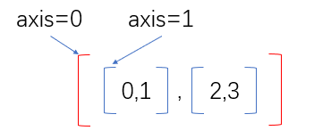
The outer bracket is axis=0, and the inner two sub brackets are axis=1.
Operation mode: if the axis is specified for relevant operations, it will use the 0th, 1st, 2nd... Of each direct child element under the axis for relevant operations respectively.

Now let's do a few operations in the way we just understood. For example, there is a two-dimensional array:

x = np.array([[0,1],[2,3]])

1. Find the sum of x array in the case of axis=0 and axis=1:

    >>> x.sum(axis=0)
    array([2, 4])
   

   The reason why we get [2,4] is that if we add it in the way of axis=0, we will add the 0th position and the first position of all direct child elements under the outermost axis... And so on, we get 0 + 2 and 2 + 3, and then add them to get [2,4].

    >>> x.sum(axis=1)
    array([1, 5])
   

   Because we add in the way of axis=1, the elements with axis 1 will be taken out for summation. The result is 0,1, which is added as 1, and 2,3 is added as 5. Therefore, the final result is [1,5].

2. Use np.max to find the maximum value when axis=0 and axis=1:

>>> np.random.seed(100)
>>> x = np.random.randint(0,10,size=(3,5))
>>> x.max(axis=0)
array([8, 8, 3, 7, 8])

Because we calculate the maximum value according to axis=0, we will find the direct child element in the outermost axis, and then put the 0th value of each child element together for the maximum value, put the first value together for the maximum value, and so on. If axis=1, we will get each direct child element and then calculate the maximum value in each child element:

>>> x.max(axis=1)
array([8, 5, 8])

1. Use np.delete to delete elements when axis=0 and axis=1:

    >>> np.delete(x,0,axis=0)
    array([[2, 3]])
   

   np.delete is an exception. If we delete by axis=0, it will first find the 0 in the direct child element under the outermost bracket, and then delete it, leaving the data in the last row.

    >>> np.delete(x,0,axis=1)
    array([[1],
           [3]])
   

   Similarly, if we delete according to axis=1, the data in the first column will be deleted.

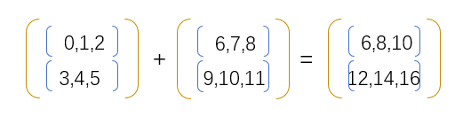
Three dimensional array:

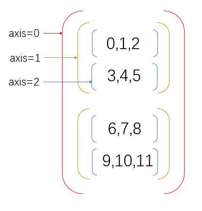
According to the previous theory, if the above arrays are added in the way of axis=0, the results are as follows:

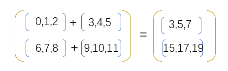
If the addition is carried out in the way of axis=1, the results are as follows:

General function

Unary function:

function	describe
np.abs	absolute value
np.sqrt	Root opening
np.square	square
np.exp	Calculate index (e^x)
np.log，np.log10，np.log2，np.log1p	Find the logarithm with e as the base, 10 as the low, 2 as the low and (1+x) as the base
np.sign	Label the values in the array. Those greater than 0 become 1, those equal to 0 become 0, and those less than 0 become - 1
np.ceil	Rounding in the direction of infinity, for example, 5.1 becomes 6 and - 6.3 becomes - 6
np.floor	Forensics in the direction of negative infinity. For example, 5.1 will become 5 and - 6.3 will become - 7
np.rint，np.round	Returns the rounded value
np.modf	Separate integers and decimals to form two arrays
np.isnan	Determine whether it is nan
np.isinf	Determine if it is inf
np.cos，np.cosh，np.sin，np.sinh，np.tan，np.tanh	trigonometric function
np.arccos，np.arcsin，np.arctan	Inverse trigonometric function

Binary function:

function	describe
np.add	Addition operation (i.e. 1 + 1 = 2), equivalent to+
np.subtract	Subtraction (i.e. 3-2 = 1), equivalent to-
np.negative	Negative number operation (i.e. - 2) is equivalent to adding a minus sign
np.multiply	Multiplication (i.e. 2 * 3 = 6), equivalent to*
np.divide	Division operation (i.e. 3 / 2 = 1.5), equivalent to/
np.floor_divide	Rounding operation, equivalent to//
np.mod	Remainder operation, equivalent to%
greater,greater_equal,less,less_equal,equal,not_equal	>, > =, <, < =, =,! = function expression
logical_and	&Function expression for
logical_or	|Function expression for

Aggregate function:

Function name	NAN Security version	describe
np.sum	np.nansum	Calculate the sum of elements
np.prod	np.nanprod	Calculate the product of elements
np.mean	np.nanmean	Calculate the average of the elements
np.std	np.nanstd	Calculate the standard deviation of the element
np.var	np.nanvar	Calculate the variance of the element
np.min	np.nanmin	Calculate the minimum value of the element
np.max	np.nanmax	Calculate the maximum value of the element
np.argmin	np.nanargmin	Find the index of the minimum value
np.argmax	np.nanargmax	Find the index of the maximum value
np.median	np.nanmedian	Calculate the median of the element

You can use np.sum or a.sum. You can specify which axis to use. Similarly, python also has a built-in sum function, but the execution efficiency of Python's built-in sum function is not as high as np.sum. You can learn from the following code test:

a = np.random.rand(1000000)
%timeit sum(a) #Use Python's built-in sum function to find the sum and see the time spent
%timeit np.sum(a) #Use Numpy's sum function to sum and look at the time it takes

Boolean array functions:

Function name	describe
np.any	Verify that any element is true
np.all	Verify that all elements are true

For example, to see if all elements in the array are 0, you can use the following code:

np.all(a==0) 
# Or
(a==0).all()

For example, if we want to see whether there is a number equal to 0 in the array, we can implement it through the following code:

np.any(a==0)
# Or
(a==0).any()

Sort:

1. np.sort: Specifies the axis for sorting. By default, the last axis of the array is used for sorting.

    a = np.random.randint(0,10,size=(3,5))
    b = np.sort(a) #Sort by row. Because the last axis is 1, the innermost elements are sorted.
    c = np.sort(a,axis=0) #Sort by column because axis=0 is specified
   

   And ndarray.sort(), which will directly affect the original array, rather than returning a new sorted array.

2. np.argsort: returns the sorted subscript value. The example code is as follows:

    np.argsort(a) #By default, the last axis is also used for sorting.
   

3. Descending sort: np.sort uses ascending sort by default. If we want to sort in descending order. Then the following scheme can be adopted:

    # 1. Use a minus sign
    -np.sort(-a)
   
    # 2. Use sort, argsort and take
    indexes = np.argsort(-a) #The sorted results are in descending order
    np.take(a,indexes) #Extract the corresponding elements from a according to the subscript
   

Other functions supplement:

1. np.apply_along_axis: executes the specified function along an axis. The example code is as follows:

    # Find the average value of array a according to rows, and remove the maximum and minimum values.
    np.apply_along_axis(lambda x:x[(x != x.max()) & (x != x.min())].mean(),axis=1,arr=a)
   

2. np.linspace: used to divide the values in the specified interval into equal parts. The example code is as follows:

    # Divide 0-1 into 12 points to generate an array
    np.linspace(0,1,12)
   

3. np.unique: returns the unique value in the array.

    # Returns the unique value in array a, and returns the number of occurrences of each unique value. np.unique(a,return_counts=True)
   

more:

https://docs.scipy.org/doc/numpy/reference/index.html

Numpy exercises

1, View Numpy's version number:

import numpy as np
print(np.__version__)

2, How to create a Boolean array with all values False:

np.full((3,3),False,dtype=np.bool)

3, Convert the shape of an array with 10 numbers:

arr = np.arange(10)
arr.reshape(2,5) #Convert to an array of (2,5)
arr[:,np.newaxis] #Convert to an array of (10,1)

The position of np.newaxis will become 1. For example:

arr = np.random.randint(0,10,size=(10,2))
arr1 = arr[:,np.newaxis,:]
print(arr1.shape)
# The result is (10,1,2), because the position of np.newaxis is 1

4, Replace all even numbers in the array with 0 (change the original array and do not change the original array):

arr = np.random.randint(0,10,size=(3,3))
# 1. Do not change the original array
arr1 = np.where(arr%2==0,0,arr)
print(arr1)
# 2. Change the original array
arr[arr%2==0] = 0

5, Create a one-dimensional array with 10 numbers. The elements are from 0 to 1, but do not contain 0 and 1:

arr = np.linspace(0,1,12)[1:-1]

The linspace is the average number of the specified number between the start value and the end value. For example, the above is to get 12 arrays from 0-1.

6, Find the following arrays greater than or equal to 5 and less than or equal to 10:

a = np.arange(15)
# Method 1
index = np.where((a >= 5) & (a <= 10))
a[index]

# Method 2:
index = np.where(np.logical_and(a>=5, a<=10))
a[index]
#> (array([6, 9, 10]),)

# Method 3:
a[(a >= 5) & (a <= 10)]

7, Reverse the rows and columns of a two-dimensional array:

a = np.arange(15).reshape(3,5)
# Reverse conversion
a1 = a[::-1] #A number is passed in (no comma appears), which means that only the line is operated
# Reverse column
a2 = a[:,::-1] #Two numbers are passed in. The first is for all rows and the second is for all columns, but the value direction is from the back to the front.

8, How to convert scientific counting to floating point printing:

# set_printoptions Used to set some configurations and options when printing# If suppress is set to True, it will not be displayed as scientific counting method, and precision is used to control how many decimal places to keep after the decimal point
np.set_printoptions(suppress=True,precision=6)
rand_arr = np.random.random([3,3])/1e3print(rand_arr)

9, Get the unique element in an array:

arr = np.random.randint(0,20,(10,10))
np.unique(arr)

10, Get the ranking of the number of unique elements in an array:

arr = np.random.randint(0,20,(10,10))
np.unique(arr,return_counts=True)

11, How to find the maximum value of each row in the array:

# Solution 1:
np.random.seed(100)
a = np.random.randint(1,10, [5,3])
print(a)
print("="*30)
print(np.amax(a,axis=1))

# Solution 2:
print(np.apply_along_axis(np.max,arr=a,axis=1))

12, How to find the result of dividing the minimum value by the maximum value according to the row:

np.random.seed(100)
a = np.random.randint(1,10, [5,3])
np.apply_along_axis(lambda x: np.min(x)/np.max(x),arr=a,axis=1)

13, Judge whether two arrays are exactly equal:

a = np.array([0,1,2])
b = np.arange(3)
(a == b).all()

14, Setting an array cannot modify the value:

a = np.zeros((2,2))
a.flags.writable = Falsea[0] = 1

15, Find the nearest value to an element in the array:

np.random.seed(100)
Z = np.random.uniform(0,1,10)
z = 0.5
m = Z[np.abs(Z - z).argmin()]
print(m)

come on.

thank!

strive!