principal component analysis
1. Summary
Principal component analysis was proposed by Karl Pearson in 1903 and improved from another perspective by Harold Hotelling in the 1930s. It is a method suitable for high-dimensional data and exploratory data analysis. As one of the first algorithms applied to pattern recognition and machine learning models, it now realizes data compression and dimensionality reduction Feature extraction is widely used in mechanics, signal processing, quality control, psychology and many other fields.
2. Algorithm idea
To put it simply: find a set of orthogonalized projections (linear transformation) maximizes the data variance of the data in the original space in the new projection space, that is, to disperse the projection results as much as possible. How to find such a linear transformation? At this time, it has to be said that the ideas of mathematicians are really unimaginable.
Suppose there is such a set of data of n samples, and each sample has d features X = { }, we centralize the data samples
 Where m is the center of all samples.
Then, in order to find the projection u of the first principal component and maximize the variance of the data in the projection space,
order , the variance D of the sample space can be expressed as:
Here m is the center of the new sample. Due to the centralization of the original data, it is easy to obtain:
be
It's not difficult Found as the skew variance matrix of the original spatial data X, where the length of the projection vector
 . The problem becomes a function:
The problem of finding the best value. Then, with the help of Lagrange multiplier method, we can convert the above function into the following form:

,
It is easy to obtain the partial derivative of u:
2Su − 2 λ u = 0, i.e. Su = λ u
Now we can see that u and λ That is, the eigenvectors and eigenvalues corresponding to matrix S one-to-one.

Therefore, solving the maximization D is to obtain the maximum eigenvalue λ, The eigenvector corresponding to the maximum eigenvalue is the "first principal component" we require. Using the same method, the eigenvalues of the easy to know matrix S covariance matrix are arranged from large to small, and the corresponding first P eigenvectors are the transformation matrix of the linear transformation.

def pca(X):
n_points, n_features = X.T.shape #to get the number of samples and the number features of each sample
mean = np.array([np.mean(X.T[:,i]) for i in range(n_features)]) #to get the mean matrix of feachures
#Centralization
cen_X = X.T-mean
#empirical covariance matrix
cov_matrix = np.dot(cen_X.T,cen_X)/(n_points-1)
#then to calculate the eigenvectors and eigenvalues using np.linalg.eig, in the numpy
eig_val, eig_vec = np.linalg.eig(cov_matrix)
res = {}
for i in range(len(eig_val)):
res[eig_val[i]] = eig_vec[i]
return eig_val, eig_vec
# Visualisation
val, vec = my_pca(X)
X=X.T
dic = {}
for i in range(len(val)):
dic[val[i]] = vec[i]
ls = sorted(dic,reverse=True)
k = 2 # to select the first 2 principal components(pc1 pc2)
new_features = np.array([dic[e] for e in ls[:k]])
print(new_features)
n_points, n_features = X.shape
mean = np.array([np.mean(X[:,i]) for i in range(n_features)])
cen_X = X-mean
print(cen_X.shape)
data=np.dot(cen_X,np.transpose(new_features))
x=[]
y = []
x.append(data.T[0])
y.append(data.T[1])
# to select the first and the third principal components(pc1 pc3)
new_features_13 = np.array([dic[ls[0]],dic[ls[2]]])
data_13=np.dot(cen_X,np.transpose(new_features_13))
x.append(data_13.T[0])
y.append(data_13.T[1])
# to select the second and the third principal components(pc2 pc3)
new_features_23 = np.array([dic[ls[1]],dic[ls[2]]])
data_23=np.dot(cen_X,np.transpose(new_features_23))
x.append(data_23.T[0])
y.append(data_23.T[1])
# to show the data sets after PCA and being projected to 2D
for i in range(len(x)):
plt.scatter(x[i],y[i])
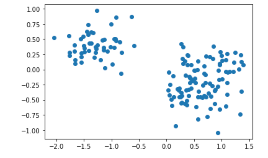
plt.show()Select different principal components to construct a linear transformation matrix for projection:
choice Compress the corresponding vector:
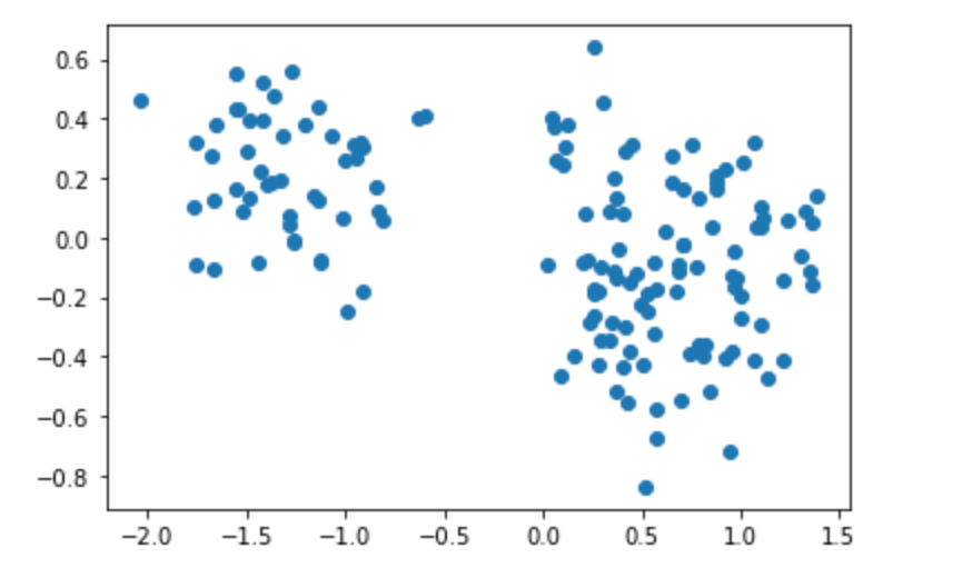
choice Compress the corresponding vector:
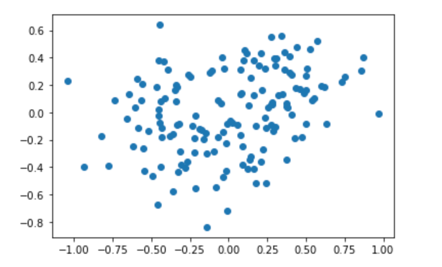
choice Compress the corresponding vector:
(dual PCA will be supplemented tomorrow)