[target detection – R-CNN, Fast R-CNN, Fast R-CNN] https://www.cnblogs.com/yanghailin/p/14767995.html
[target detection SSD] https://www.cnblogs.com/yanghailin/p/14769384.html
[detailed explanation of anchor generation of ssd] https://www.cnblogs.com/yanghailin/p/14868575.html
[detailed explanation of ssd network] https://www.cnblogs.com/yanghailin/p/14871296.html
[detailed explanation of ssd loss] https://www.cnblogs.com/yanghailin/p/14882807.html
In fact, I read the ssd source code a while ago and wrote the above blog. Then I don't remember it at all after a while... Then I read it again recently, but this time I read the source code much faster,
In particular, there is a further understanding of some previously ambiguous places.
ssd network part
I wrote it again...
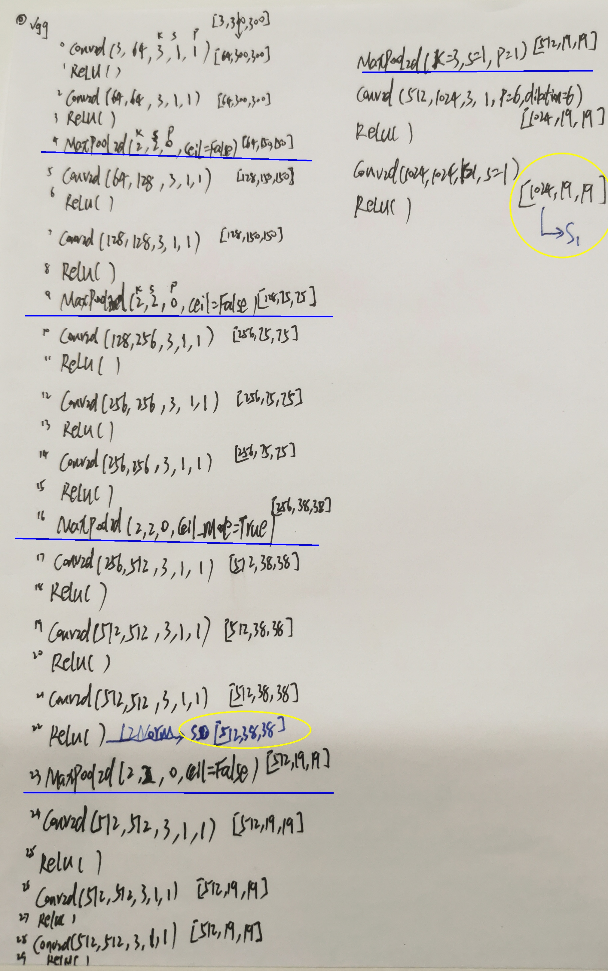
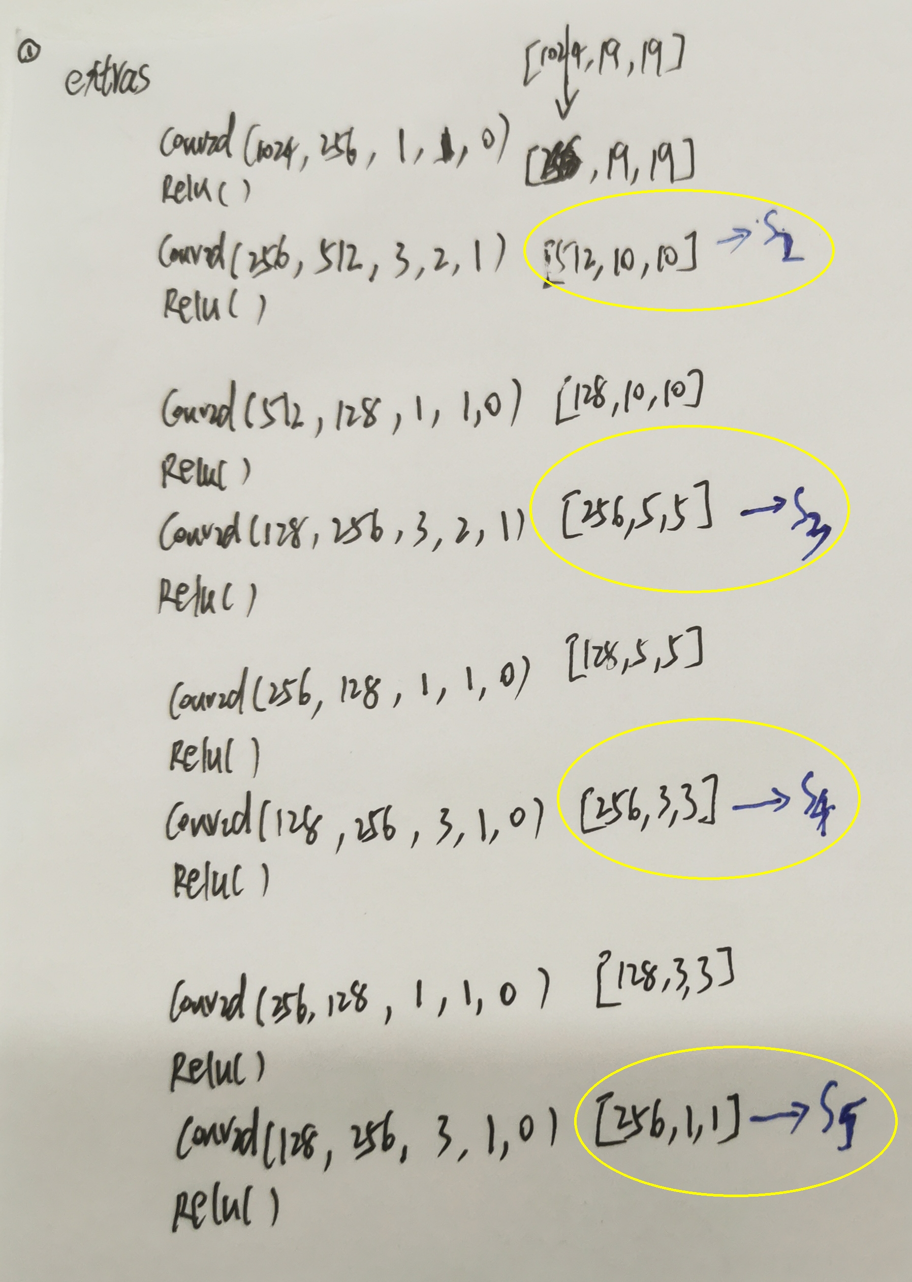
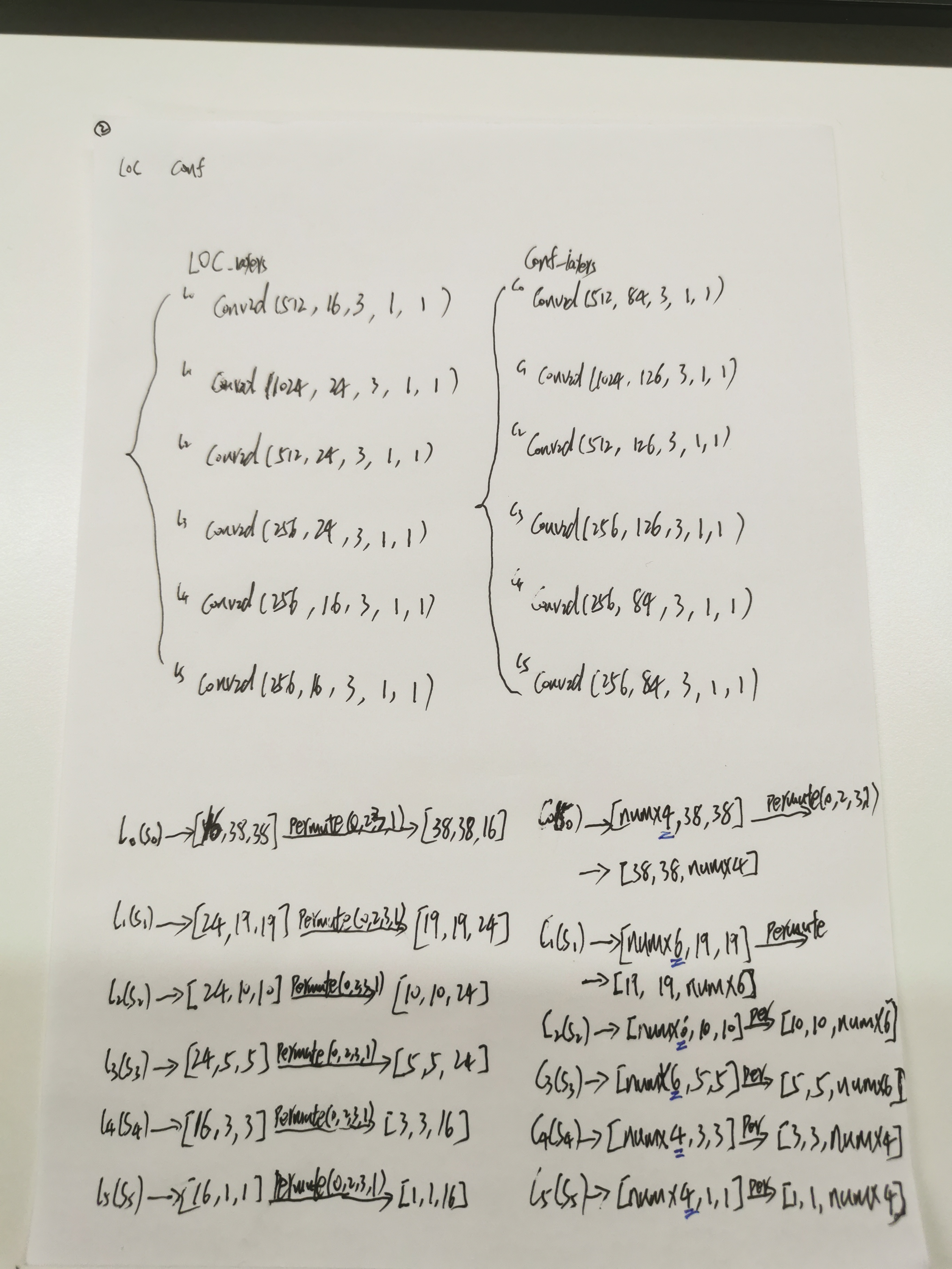
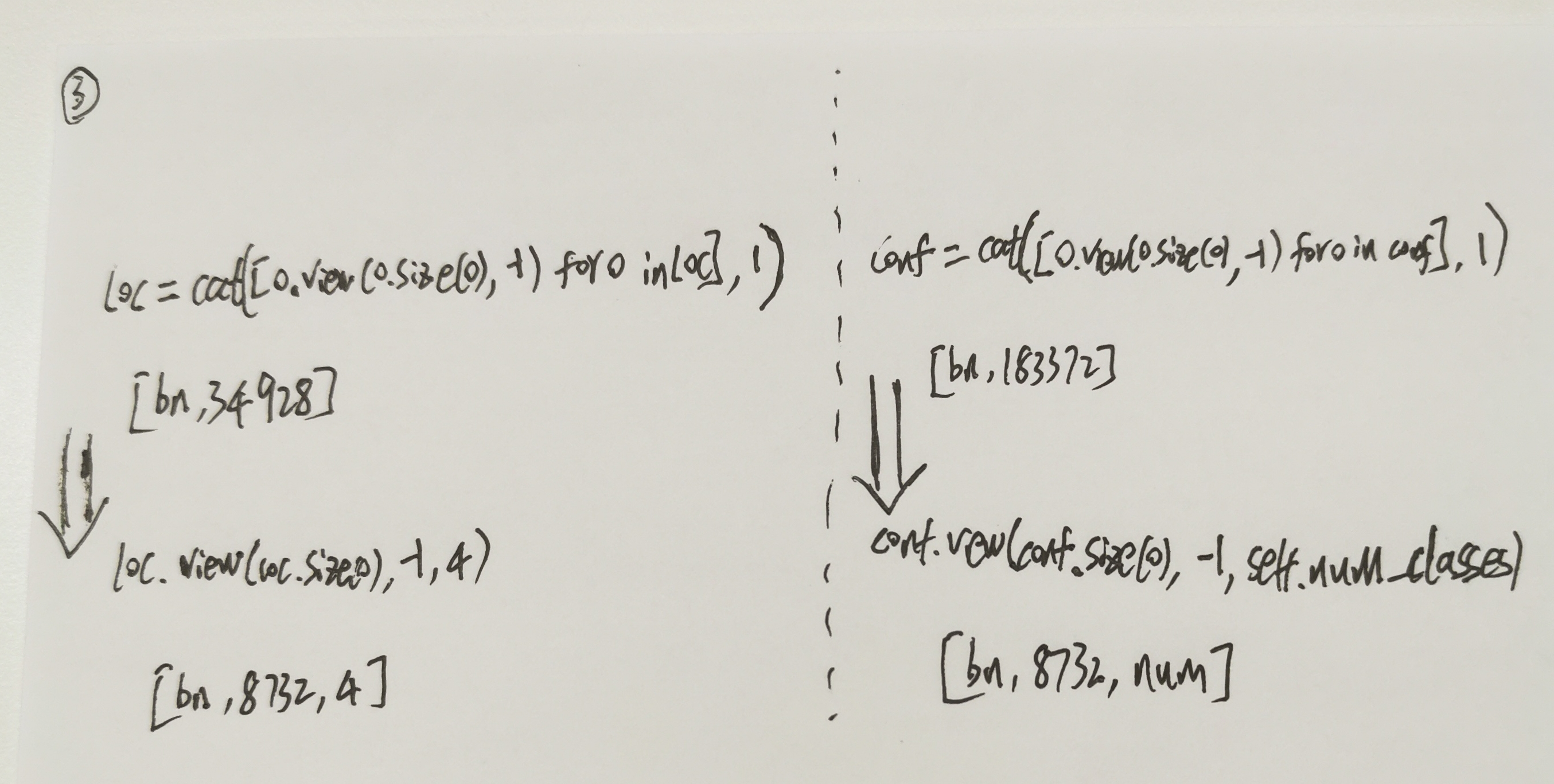
The above diagram I wrote according to the code is consistent with the diagram in the paper:

Last LOC above me [BN, 8732,4]
conf [bn,8732,num]
Is the output of the network.
ssd loss part – ssd codec
As for codec, I was confused when I first read it. That's what you say. The formula in the ssd paper is as follows:
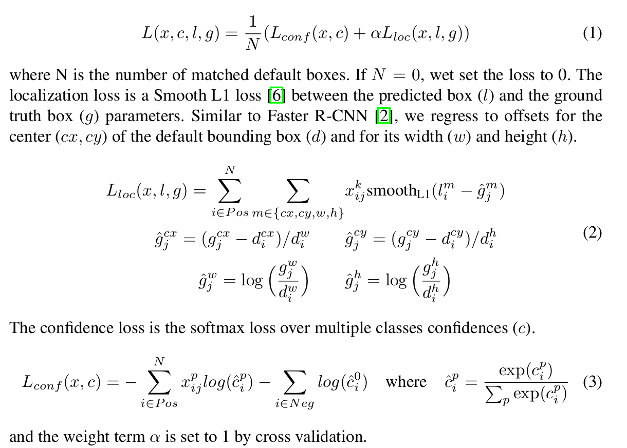
Then I saw a detailed introduction in fast RCNN.
https://blog.csdn.net/weixin_42782150/article/details/110522380
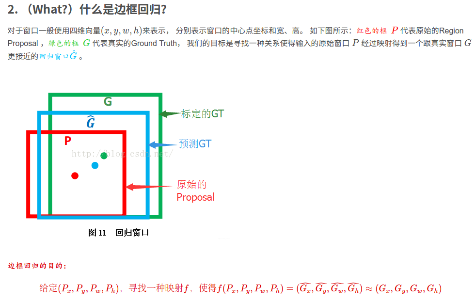
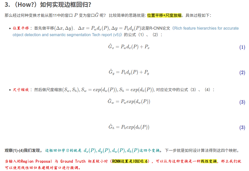
In order to make the predicted frame close to gt, you need to add an offset to the anchor frame center point x and y, and multiply the width and height by a coefficient, which is not 0! Close to gt, so this mathematical formula came into being.
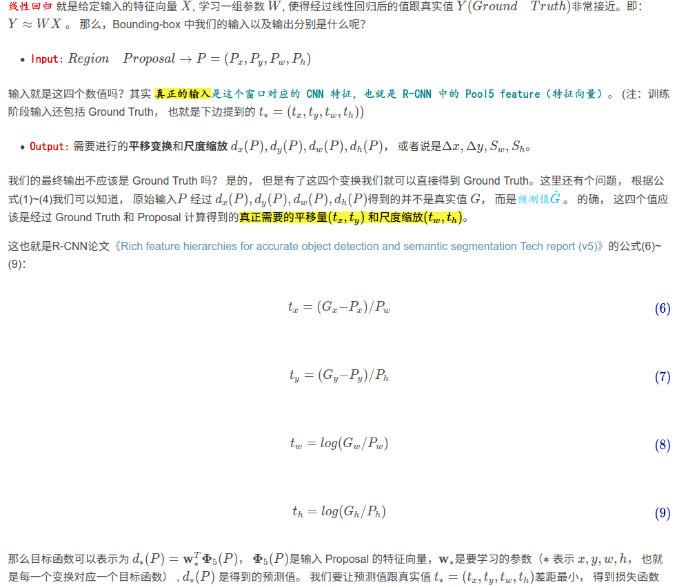
In the fast RCNN paper:
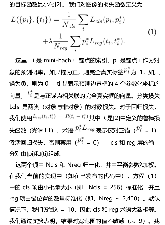
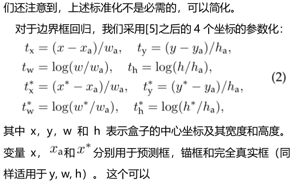
You can see that there are two sets of t and t *
I didn't understand it at first, but then I realized it in the wilderness!
The following T formula is the offset between gt and anchor. E-learning is such an offset t! Look at the loss formula above, which is t and t. The purpose is to bring the network closer to t *.
t is after coding, and this coding relationship is shown in the above formula.
About how to calculate intersection and union ratio, I don't see the operation of mapping to the original graph.
When calculating intersection ratio, I don't see a for loop.
def point_form(boxes):
    """ Convert prior_boxes to (xmin, ymin, xmax, ymax)
    representation for comparison to point form ground truth data.
    Args:
        boxes: (tensor) center-size default boxes from priorbox layers.
    Return:
        boxes: (tensor) Converted xmin, ymin, xmax, ymax form of boxes.
    """
    return torch.cat((boxes[:, :2] - boxes[:, 2:]/2,     # xmin, ymin
                     boxes[:, :2] + boxes[:, 2:]/2), 1)  # xmax, ymax
def intersect(box_a, box_b):
    """ We resize both tensors to [A,B,2] without new malloc:
    [A,2] -> [A,1,2] -> [A,B,2]
    [B,2] -> [1,B,2] -> [A,B,2]
    Then we compute the area of intersect between box_a and box_b.
    Args:
      box_a: (tensor) bounding boxes, Shape: [A,4].
      box_b: (tensor) bounding boxes, Shape: [B,4].
    Return:
      (tensor) intersection area, Shape: [A,B].
    """
    A = box_a.size(0)
    B = box_b.size(0)

    # n1 = box_a[:, 2:]
    # n1_1 = box_a[:, 2:].unsqueeze(1)
    # n1_2 = box_a[:, 2:].unsqueeze(1).expand(A, B, 2)
    #
    # n2 = box_b[:, 2:]
    # n2_1 = box_b[:, 2:].unsqueeze(0)
    # n2_2 = box_b[:, 2:].unsqueeze(0).expand(A, B, 2)
    #
    # n3 = torch.min(n1_2, n2_2)

    max_xy = torch.min(box_a[:, 2:].unsqueeze(1).expand(A, B, 2),
                       box_b[:, 2:].unsqueeze(0).expand(A, B, 2))
    min_xy = torch.max(box_a[:, :2].unsqueeze(1).expand(A, B, 2),
                       box_b[:, :2].unsqueeze(0).expand(A, B, 2))

    # sub_ = max_xy - min_xy

    inter = torch.clamp((max_xy - min_xy), min=0)
    return inter[:, :, 0] * inter[:, :, 1]


def jaccard(box_a, box_b):
    """Compute the jaccard overlap of two sets of boxes.  The jaccard overlap
    is simply the intersection over union of two boxes.  Here we operate on
    ground truth boxes and default boxes.
    E.g.:
        A ∩ B / A ∪ B = A ∩ B / (area(A) + area(B) - A ∩ B)
    Args:
        box_a: (tensor) Ground truth bounding boxes, Shape: [num_objects,4]
        box_b: (tensor) Prior boxes from priorbox layers, Shape: [num_priors,4]
    Return:
        jaccard overlap: (tensor) Shape: [box_a.size(0), box_b.size(0)]
    """
    inter = intersect(box_a, box_b)
    area_a = ((box_a[:, 2]-box_a[:, 0]) *
              (box_a[:, 3]-box_a[:, 1])).unsqueeze(1).expand_as(inter)  # [A,B]
    area_b = ((box_b[:, 2]-box_b[:, 0]) *
              (box_b[:, 3]-box_b[:, 1])).unsqueeze(0).expand_as(inter)  # [A,B]
    union = area_a + a
    rea_b - inter
    return inter / union  # [A,B]

overlaps = jaccard(
        truths,
        point_form(priors)
    )
After looking at the code, all operations are relative values, values between 0-1. This value multiplied by the size of the original image can be mapped to the original image, so the code is a relative value, which is consistent with the operation on the original image.
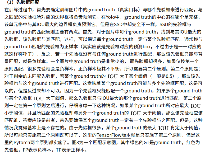
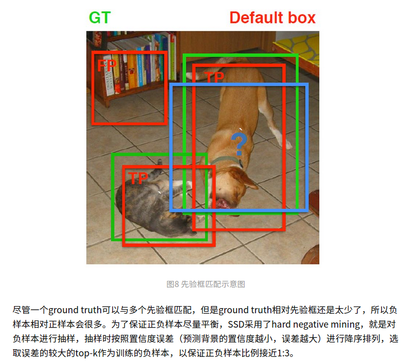
A priori box matching rule
When calculating the intersection and comparison between gt and anchor. There are very few gt in a graph. There are 1,2 targets and 8732 anchor.
The strategy in the code is to ensure that a gt matches the anchor with the largest intersection and union ratio, and then each anchor matches a gt with the largest intersection and union ratio!

Look at this figure, first find the one with the largest gt and anchor horizontally. This is the highest priority, and there is logic to ensure that this is always satisfied.
 best_truth_overlap.index_fill_(0, best_prior_idx, 2)  # ensure best prior
    # TODO refactor: index  best_prior_idx with long tensor
    # ensure every gt matches with its prior of max overlap
    for j in range(best_prior_idx.size(0)):
        best_truth_idx[best_prior_idx[j]] = j
Find the maximum longitudinally, that is, the gt corresponding to the maximum intersection union ratio of each anchor. Then 8732 anchors are encoded with matching gt.
The set background class whose intersection and union ratio of anchor and gt is less than a certain threshold.
My blog has analyzed:
https://www.cnblogs.com/yanghailin/p/14882807.html
This knowledge has an explanation about a priori frame matching: https://zhuanlan.zhihu.com/p/33544892
Difficult case excavation:
It's hard. I still don't understand one paragraph. But I feel the design is very clever! sort twice.
 #loss_c[26196,1]    #https://zhuanlan.zhihu.com/p/153535799
loss_c = log_sum_exp(batch_conf) - batch_conf.gather(1, conf_t.view(-1, 1))
Here I release the code with detailed comments
# -*- coding: utf-8 -*-
import torch
import torch.nn as nn
import torch.nn.functional as F
from torch.autograd import Variable
from data import coco as cfg
from ..box_utils import match, log_sum_exp

# criterion = MultiBoxLoss(cfg['num_classes'], 0.5, True, 0, True, 3, 0.5,
#                          False, args.cuda)

class MultiBoxLoss(nn.Module):
    """SSD Weighted Loss Function
    Compute Targets:
        1) Produce Confidence Target Indices by matching  ground truth boxes
           with (default) 'priorboxes' that have jaccard index > threshold parameter
           (default threshold: 0.5).
        2) Produce localization target by 'encoding' variance into offsets of ground
           truth boxes and their matched  'priorboxes'.
        3) Hard negative mining to filter the excessive number of negative examples
           that comes with using a large number of default bounding boxes.
           (default negative:positive ratio 3:1)
    Objective Loss:
        L(x,c,l,g) = (Lconf(x, c) + αLloc(x,l,g)) / N
        Where, Lconf is the CrossEntropy Loss and Lloc is the SmoothL1 Loss
        weighted by α which is set to 1 by cross val.
        Args:
            c: class confidences,
            l: predicted boxes,
            g: ground truth boxes
            N: number of matched default boxes
        See: https://arxiv.org/pdf/1512.02325.pdf for more details.
    """

    def __init__(self, num_classes, overlap_thresh, prior_for_matching,
                 bkg_label, neg_mining, neg_pos, neg_overlap, encode_target,
                 use_gpu=True):
        super(MultiBoxLoss, self).__init__()
        self.use_gpu = use_gpu
        self.num_classes = num_classes
        self.threshold = overlap_thresh
        self.background_label = bkg_label
        self.encode_target = encode_target
        self.use_prior_for_matching = prior_for_matching
        self.do_neg_mining = neg_mining
        self.negpos_ratio = neg_pos
        self.neg_overlap = neg_overlap
        self.variance = cfg['variance']

    def forward(self, predictions, targets):
        """Multibox Loss
        Args:
            predictions (tuple): A tuple containing loc preds, conf preds,
            and prior boxes from SSD net.
                conf shape: torch.size(batch_size,num_priors,num_classes)
                loc shape: torch.size(batch_size,num_priors,4)
                priors shape: torch.size(num_priors,4)

            targets (tensor): Ground truth boxes and labels for a batch,
                shape: [batch_size,num_objs,5] (last idx is the label).

                loc_data [3,8732,4]
                conf_data [3,8732,21]
                priors [8732,4]
        """
        loc_data, conf_data, priors = predictions
        num = loc_data.size(0) # num is batchsize
        priors = priors[:loc_data.size(1), :] #priors [8732,4]
        num_priors = (priors.size(0)) #num_priors=8732
        num_classes = self.num_classes #21

        # match priors (default boxes) and ground truth boxes
        loc_t = torch.Tensor(num, num_priors, 4) #[3,8732,4]
        conf_t = torch.LongTensor(num, num_priors) #[3,8732]
        for idx in range(num):
            truths = targets[idx][:, :-1].data
            labels = targets[idx][:, -1].data
            defaults = priors.data
            match(self.threshold, truths, defaults, self.variance, labels,
                  loc_t, conf_t, idx)
        if self.use_gpu:
            loc_t = loc_t.cuda()
            conf_t = conf_t.cuda()

        #Suffix_ The variable of t represents truth
        #The LOC obtained from match here_ t[3,8732,4], conf_t[3,8732]
        #loc_ T [38732,4] is the value after encoding each anchor and gt
        #conf_t[3, 8732] is the value between label, 0-21, which is 0 in most places. There is a value only where the intersection ratio of anchor and gt is greater than the threshold
        # wrap targets
        loc_t = Variable(loc_t, requires_grad=False) #[3,8732,4]
        conf_t = Variable(conf_t, requires_grad=False) #[3,8732]

        # POS [38732] false, true is important! Select the positive sample position. The positive sample position is true and the rest are false
        # num_ POS shape [3,1] | [23], [4], [9] number of positive samples per graph
        pos = conf_t > 0 #pos [3,8732]  False,True
        num_pos = pos.sum(dim=1, keepdim=True) #num_pos shape[3,1]   | [23],[4],[9]


        # Localization Loss (Smooth L1)
        #pos [3,8732]
        #pos.dim()=2
        #pos.unsqueeze(pos.dim()) [3,8732,1]
        # loc_data [3,8732,4]
        # pos_ IDX [38732,4] True False 𞓜 is to enlarge the True and False in POS to [38732,4]
        pos_idx = pos.unsqueeze(pos.dim()).expand_as(loc_data)

        #loc_data[3, 8732, 4]   aa[144]
        aa = loc_data[pos_idx]
        #[3,8732,4]   bb[144]
        bb = loc_t[pos_idx]

        #pos_idx [3,8732,4] True  False
        #loc_ Data [38732,4] network prediction output value
        #loc_data[pos_idx] shape[144]  (23+4+9)×4=144
        # loc_t [3,8732,4]
        #loc_t[pos_idx] shape[144]  (23+4+9)×4=144
        loc_p = loc_data[pos_idx].view(-1, 4)
        loc_t = loc_t[pos_idx].view(-1, 4)
        #loss_l tensor(14.0165, grad_fn=<SmoothL1LossBackward>)
        loss_l = F.smooth_l1_loss(loc_p, loc_t, size_average=False)

        # Compute max conf across batch for hard negative mining
        #conf_ Data [38732,21] network prediction value
        # batch_conf[3*8732,21]  [26196,21]
        # tt_1 = batch_conf.max() ## 35
        # tt_2 = batch_conf.min() ## -13
        #The maximum and minimum values are taken out here. It is convenient and intuitive to feel what the values are. You can see that this value is actually used to predict the label. Without softmax
        batch_conf = conf_data.view(-1, self.num_classes)

        b1 = log_sum_exp(batch_conf) #[26196,1]
        # conf_t[3,8732]
        # conf_t.view(-1, 1) [26196,1]
        b2 = batch_conf.gather(1, conf_t.view(-1, 1)) #[26196,1]


        #https://blog.csdn.net/liyu0611/article/details/100547145
        #https://zhuanlan.zhihu.com/p/35709485
        # https://zhuanlan.zhihu.com/p/153535799
        #loss_c[26196,1]
        loss_c = log_sum_exp(batch_conf) - batch_conf.gather(1, conf_t.view(-1, 1))

        # Hard Negative Mining
        #loss_c[pos] = 0  # filter out pos boxes for now
        #loss_c = loss_c.view(num, -1)
        #loss_c [3,8732]
        loss_c = loss_c.view(num, -1)
        #pos [3,8732]
        # loss_c [3,8732]
        loss_c[pos] = 0 #Set the loss of the positive sample to 0

        #Twice sort https://blog.csdn.net/laizi_laizi/article/details/103482634
        #loss_idx [3,8732]
        tmp1, loss_idx = loss_c.sort(1, descending=True) ## _, loss_idx = loss_c.sort(1, descending=True)
        #idx_rank [3,8732]
        tmp2, idx_rank = loss_idx.sort(1) ## _, idx_rank = loss_idx.sort(1)

        # pos [3,8732]
        # num_pos shape[3,1]   | [23],[4],[9]
        num_pos = pos.long().sum(1, keepdim=True)

        # aaaaa shape[3,1]   | [23*3],[4*3],[9*3]
        #aaaaa = self.negpos_ratio * num_pos
        # num_neg shape[3,1]   | [23*3],[4*3],[9*3]
        num_neg = torch.clamp(self.negpos_ratio*num_pos, max=pos.size(1)-1)#num_pos shape[3,1]   | [69],[12],[27]

        # num_neg shape[3,1]
        # idx_rank[3,8732]
        #Neg [38732] True, False gives loss_c is sorted from large to small by True and False of corresponding coordinates
        neg = idx_rank < num_neg.expand_as(idx_rank)
        # Confidence Loss Including Positive and Negative Examples
        # pos[3,8732]
        # pos.unsqueeze(2)  [3,8732,1]
        #conf_data[3, 8732, 21]
        #pos_idx [3, 8732, 21]
        pos_idx = pos.unsqueeze(2).expand_as(conf_data)#pos[3,8732]  conf_data[3,8732,21]
        # neg [3,8732]
        # neg_idx [3, 8732, 21]
        neg_idx = neg.unsqueeze(2).expand_as(conf_data)##neg [3,8732]  conf_data[3,8732,21]


        # tmp_1111 = pos_idx + neg_idx #[3,8732,21]  True  False   ##Other POS_ idx+neg_ The shapes of IDX and IDX are the same [38732,21]. The values are True or False. The addition operation is equivalent to the or operation. As long as there is one True, it is True
        # tmp_2222 = (pos_idx+neg_idx).gt(0) #[3,8732,21]  True  False
        # conf_data [3,8732,21]
        # tmp_333 = conf_data[(pos_idx + neg_idx).gt(0)] #[3696]
        #conf_p [176,21]          #Other conf_ P [144,21] -- > the 144 is the above two pos_idx and neg_ Sum of True quantities in IDX 69 + 12 + 27 + 23 + 4 + 9 = 144
        conf_p = conf_data[(pos_idx+neg_idx).gt(0)].view(-1, self.num_classes)
        # pos [3,8732]
        # neg [3,8732]
        # conf_t [3,8732]
        # targets_weighted  [176]   ||[144]
        targets_weighted = conf_t[(pos+neg).gt(0)]
        #loss_c tensor(58.0656, grad_fn=<NllLossBackward>)
        loss_c = F.cross_entropy(conf_p, targets_weighted, size_average=False)

        # Sum of losses: L(x,c,l,g) = (Lconf(x, c) + αLloc(x,l,g)) / N

        N = num_pos.data.sum() ##N=36 is num_ Sum of POS [23] + [4] + [9]
        loss_l /= N
        loss_c /= N
        return loss_l, loss_c
There are two things to say:
The first place is
loss_c = log_sum_exp(batch_conf) - batch_conf.gather(1, conf_t.view(-1, 1))
This actually feels like cross entropy, log_sum_exp is the minus sign after the following formula, batch_conf.gather(1, conf_t.view(-1, 1)) is xj
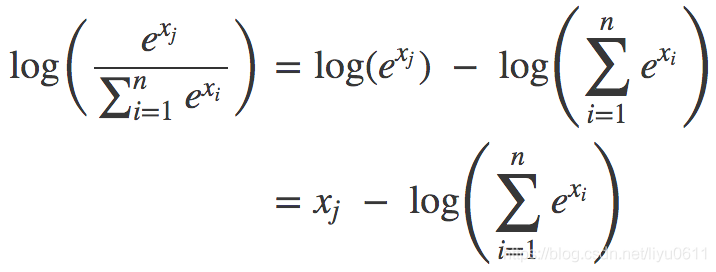
The formula comes from the following blog.
https://blog.csdn.net/liyu0611/article/details/100547145
Why log_sum_exp, because the 1000th power of e will exceed the numerical expression range. Look specifically https://zhuanlan.zhihu.com/p/153535799
I just don't understand the following:
loss_c = log_sum_exp(batch_conf) - batch_conf.gather(1, conf_t.view(-1, 1))
loss_c = F.cross_entropy(conf_p, targets_weighted, size_average=False)
What's the difference? Why did you write that first.
There are two sort s
https://blog.csdn.net/laizi_laizi/article/details/103482634
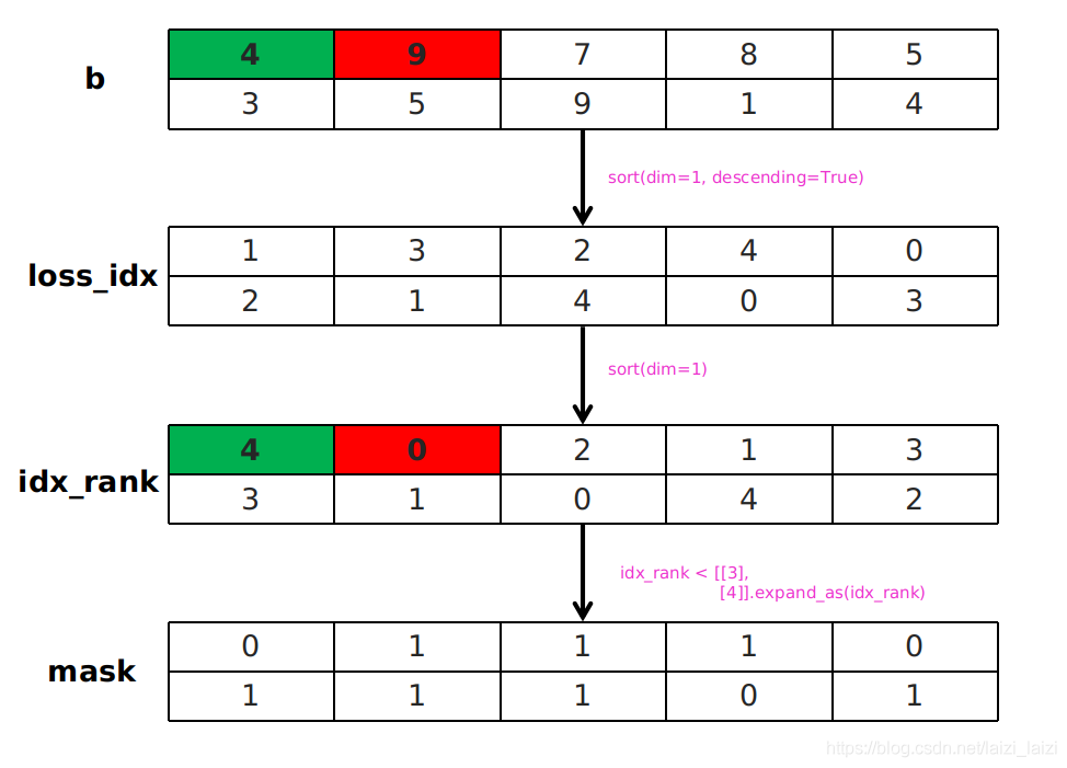
This picture is very clear. The purpose of twice sort is to easily take out the top number of values and get its position. Very severe!