catalogue
1. Monthly analysis of consumption
5. Analysis of repurchase rate and repurchase rate
6. Commodity Association Rule Mining
1, Project background
Detailed data of consumer goods sales obtained by "scanning" the bar code of individual products at the electronic point of sale of retail stores. These data provide detailed information about the quantity, characteristics, value and price of the goods sold.
2, Data source
https://www.kaggle.com/marian447/retail-store-sales-transactions
3, Ask questions
- Consumption analysis and user purchase mode analysis
- RFM and CLV analysis
- Mining association rules of different categories of goods
4, Understanding data
- Date: purchase date
- Customer_ User ID: user ID
- Transaction_ID: transaction ID
- SKU_Category: SKU code of commodity classification
- SKU: the unique SKU code of the product
- Quantity: purchase quantity
- Sales_Amount: purchase amount
5, Data cleaning
1. Import data
In [1]:
import numpy as np
import pandas as pd
from matplotlib import pyplot as plt
import seaborn as sns
%matplotlib inline
# Change design style
plt.style.use('ggplot')
plt.rcParams['font.sans-serif'] = ['SimHei']
In [2]:
df = pd.read_csv('E:/googledownload/archive (5)/scanner_data.csv')
df.head()
Out[2]:
| Unnamed: 0 | Date | Customer_ID | Transaction_ID | SKU_Category | SKU | Quantity | Sales_Amount | |
|---|---|---|---|---|---|---|---|---|
| 0 | 1 | 2017-01-02 | 2547 | 1 | X52 | 0EM7L | 1.0 | 3.13 |
| 1 | 2 | 2017-01-02 | 822 | 2 | 2ML | 68BRQ | 1.0 | 5.46 |
| 2 | 3 | 2017-01-02 | 3686 | 3 | 0H2 | CZUZX | 1.0 | 6.35 |
| 3 | 4 | 2017-01-02 | 3719 | 4 | 0H2 | 549KK | 1.0 | 5.59 |
| 4 | 5 | 2017-01-02 | 9200 | 5 | 0H2 | K8EHH | 1.0 | 6.88 |
In [3]:
df.info()
<class 'pandas.core.frame.DataFrame'>
RangeIndex: 131706 entries, 0 to 131705
Data columns (total 8 columns):
 #   Column          Non-Null Count   Dtype
---  ------          --------------   -----
 0   Unnamed: 0      131706 non-null  int64
 1   Date            131706 non-null  object
 2   Customer_ID     131706 non-null  int64
 3   Transaction_ID  131706 non-null  int64
 4   SKU_Category    131706 non-null  object
 5   SKU             131706 non-null  object
 6   Quantity        131706 non-null  float64
 7   Sales_Amount    131706 non-null  float64
dtypes: float64(2), int64(3), object(3)
memory usage: 8.0+ MB
2. Select subset
The first column is the data number, which has been indexed, so it is deleted
In [4]:
df.drop(columns='Unnamed: 0', inplace=True)
df.info()
<class 'pandas.core.frame.DataFrame'>
RangeIndex: 131706 entries, 0 to 131705
Data columns (total 7 columns):
 #   Column          Non-Null Count   Dtype
---  ------          --------------   -----
 0   Date            131706 non-null  object
 1   Customer_ID     131706 non-null  int64
 2   Transaction_ID  131706 non-null  int64
 3   SKU_Category    131706 non-null  object
 4   SKU             131706 non-null  object
 5   Quantity        131706 non-null  float64
 6   Sales_Amount    131706 non-null  float64
dtypes: float64(2), int64(2), object(3)
memory usage: 7.0+ MB
3. Delete duplicate values
In [5]:
df.duplicated().sum()
Out[5]:
0
Data has no duplicate value
4. Missing value processing
In [6]:
df.isnull().sum()
Out[6]:
Date              0
Customer_ID       0
Transaction_ID    0
SKU_Category      0
SKU               0
Quantity          0
Sales_Amount      0
dtype: int64
There is no missing value in the data
5. Standardized treatment
In [7]:
df.dtypes
Out[7]:
Date               object
Customer_ID         int64
Transaction_ID      int64
SKU_Category       object
SKU                object
Quantity          float64
Sales_Amount      float64
dtype: object
Date is an object type and needs to be standardized into date type format
In [8]:
df.Date = pd.to_datetime(df.Date, format='%Y-%m-%d')
df.dtypes
Out[8]:
Date              datetime64[ns]
Customer_ID                int64
Transaction_ID             int64
SKU_Category              object
SKU                       object
Quantity                 float64
Sales_Amount             float64
dtype: object
6. Abnormal value handling
In [9]:
df[['Quantity','Sales_Amount']].describe()
Out[9]:
| Quantity | Sales_Amount | |
|---|---|---|
| count | 131706.000000 | 131706.000000 |
| mean | 1.485311 | 11.981524 |
| std | 3.872667 | 19.359699 |
| min | 0.010000 | 0.020000 |
| 25% | 1.000000 | 4.230000 |
| 50% | 1.000000 | 6.920000 |
| 75% | 1.000000 | 12.330000 |
| max | 400.000000 | 707.730000 |
The purchase quantity is less than 1 because the weighing unit is less than 1, which is not an abnormal value
6, Analysis content
1. Monthly analysis of consumption
(1) Trend analysis of total monthly consumption
In [10]:
df['Month'] = df.Date.astype('datetime64[M]')
df.head()
Out[10]:
| Date | Customer_ID | Transaction_ID | SKU_Category | SKU | Quantity | Sales_Amount | Month | |
|---|---|---|---|---|---|---|---|---|
| 0 | 2017-01-02 | 2547 | 1 | X52 | 0EM7L | 1.0 | 3.13 | 2017-01-01 |
| 1 | 2017-01-02 | 822 | 2 | 2ML | 68BRQ | 1.0 | 5.46 | 2017-01-01 |
| 2 | 2017-01-02 | 3686 | 3 | 0H2 | CZUZX | 1.0 | 6.35 | 2017-01-01 |
| 3 | 2017-01-02 | 3719 | 4 | 0H2 | 549KK | 1.0 | 5.59 | 2017-01-01 |
| 4 | 2017-01-02 | 9200 | 5 | 0H2 | K8EHH | 1.0 | 6.88 | 2017-01-01 |
In [11]:
grouped_month = df.groupby('Month')
In [12]:
grouped_month.Sales_Amount.sum()
Out[12]:
Month
2017-01-01    111200.28
2017-02-01    118323.24
2017-03-01    126770.11
2017-04-01    140114.18
2017-05-01    141536.95
2017-06-01    130384.85
2017-07-01    124357.15
2017-08-01    114295.16
2017-09-01    139665.01
2017-10-01    141692.79
2017-11-01    131676.89
2017-12-01    156308.81
2018-01-01      1713.20
Name: Sales_Amount, dtype: float64
The data of January 2018 may be incomplete and will not be included in the trend analysis
In [13]:
grouped_month.Sales_Amount.sum().head(12).plot()
Out[13]:
<matplotlib.axes._subplots.AxesSubplot at 0x1e990450a20>
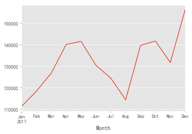
- It can be seen from the above figure that the consumption amount fluctuates greatly, which keeps rising in the first quarter, and fluctuates greatly in the follow-up, showing an upward trend as a whole
(2) Trend analysis of monthly transaction times
In [14]:
grouped_month.Transaction_ID.nunique().head(12).plot()
Out[14]:
<matplotlib.axes._subplots.AxesSubplot at 0x1e9905160f0>
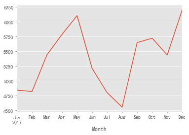
- It can be seen from the above figure that the trading times fluctuated greatly and showed an upward trend in the early stage. After May, the trading times began to decline, fell to the lowest value in August, and then began to fluctuate and recover, and returned to the peak in December
(3) Trend analysis of monthly commodity purchase quantity
In [15]:
grouped_month.Quantity.sum().head(12).plot()
Out[15]:
<matplotlib.axes._subplots.AxesSubplot at 0x1e990c9f9e8>
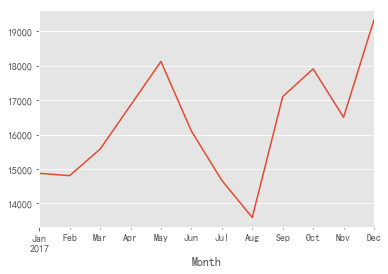
- It can be seen from the above figure that the quantity of goods purchased fluctuates greatly, and the overall trend is consistent with the number of transactions
(4) Monthly consumption trend analysis
In [16]:
grouped_month.Customer_ID.nunique().head(12).plot()
Out[16]:
<matplotlib.axes._subplots.AxesSubplot at 0x1e990d10048>
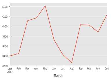
- It can be seen from the above figure that the monthly number of buyers can be divided into three stages: from January to may, from June to August, and from September to December, it shows a fluctuating upward trend
2. User distribution analysis
(1) New user distribution
In [17]:
grouped_customer = df.groupby('Customer_ID')
grouped_customer.Date.min().value_counts().plot()
Out[17]:
<matplotlib.axes._subplots.AxesSubplot at 0x1e990fc3eb8>
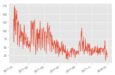
- It can be seen from the above figure that the acquisition of new users is unstable and fluctuates greatly, with a slight downward trend as a whole
In [18]:
grouped_customer.Month.min().value_counts().plot()
Out[18]:
<matplotlib.axes._subplots.AxesSubplot at 0x1e991149ef0>
- As can be seen from the above figure: according to monthly statistics, the number of new users per month has an obvious downward trend. It shows that the acquisition of new users is in a sharp downward trend, which needs attention. Appropriately increase marketing activities to improve the acquisition of new users
(2) Analysis on the proportion of one-time consumption and multiple consumption users
In [19]:
#Proportion of users who consume only once
(grouped_customer.Transaction_ID.nunique() == 1).sum()/df.Customer_ID.nunique()
Out[19]:
0.5098342541436464
- According to the calculation, half of the users only consume once
In [20]:
grouped_month_customer = df.groupby(['Month', 'Customer_ID'])
In [21]:
#The first purchase time of each user every month
data_month_min_date = grouped_month_customer.Date.min().reset_index()
#First purchase time of each user
data_min_date = grouped_customer.Date.min().reset_index()
In [22]:
#Through Customer_ID simultaneous two tables
merged_date = pd.merge(data_month_min_date, data_min_date, on='Customer_ID')
merged_date.head()
Out[22]:
| Month | Customer_ID | Date_x | Date_y | |
|---|---|---|---|---|
| 0 | 2017-01-01 | 1 | 2017-01-22 | 2017-01-22 |
| 1 | 2017-01-01 | 3 | 2017-01-02 | 2017-01-02 |
| 2 | 2017-01-01 | 11 | 2017-01-29 | 2017-01-29 |
| 3 | 2017-01-01 | 12 | 2017-01-07 | 2017-01-07 |
| 4 | 2017-01-01 | 13 | 2017-01-11 | 2017-01-11 |
In [23]:
#Date_x equals Date_y is the new user every month
((merged_date.query('Date_x == Date_y')).groupby('Month').Customer_ID.count() / merged_date.groupby('Month').Customer_ID.count()).plot()
Out[23]:
<matplotlib.axes._subplots.AxesSubplot at 0x1e991202cf8>
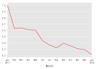
- It can be seen from the above figure that the proportion of new users per month shows a downward trend as a whole. Combined with the trend of monthly consumption, the consumption has an upward trend in the fourth quarter, so the number of re purchases has increased during the period
3. User layered analysis
(1) RFM layered analysis
In [24]:
pivot_rfm = df.pivot_table(index='Customer_ID',
              values=['Date', 'Transaction_ID', 'Sales_Amount'],
              aggfunc={'Date':'max', 'Transaction_ID':'nunique', 'Sales_Amount':'sum'})
In [25]:
pivot_rfm['R'] = (pivot_rfm.Date.max() - pivot_rfm.Date)/np.timedelta64(1, 'D')
pivot_rfm.rename(columns={'Transaction_ID':'F', 'Sales_Amount':'M'}, inplace=True)
In [26]:
def label_func(data):
    label = data.apply(lambda x:'1' if x > 0 else '0')
    label = label.R + label.F + label.M
    labels = {
        '111':'Important value customers',
        '011':'Important to keep customers',
        '101':'Key development customers',
        '001':'Important retention customers',
        '110':'General value customers',
        '010':'General customer retention',
        '100':'General development customers',
        '000':'General retention of customers'
    }
    return labels[label]
pivot_rfm['label'] = pivot_rfm[['R','F','M']].apply(lambda x:x-x.mean()).apply(label_func, axis=1)
In [27]:
pivot_rfm.label.value_counts().plot.barh()
Out[27]:
<matplotlib.axes._subplots.AxesSubplot at 0x1e9914a5f98>
In [28]:
pivot_rfm.groupby('label').M.sum().plot.pie(figsize=(6,6), autopct='%3.2f%%')
Out[28]:
<matplotlib.axes._subplots.AxesSubplot at 0x1e991b29d30>
In [29]:
pivot_rfm.groupby('label').agg(['sum', 'count'])
Out[29]:
| M | F | R | ||||
|---|---|---|---|---|---|---|
| sum | count | sum | count | sum | count | |
| label | ||||||
| General value customers | 38702.46 | 991 | 3653 | 991 | 258396.0 | 991 |
| General customer retention | 75475.62 | 1802 | 7161 | 1802 | 97961.0 | 1802 |
| General development customers | 144065.48 | 8329 | 10089 | 8329 | 2256955.0 | 8329 |
| General retention of customers | 119097.65 | 6313 | 8158 | 6313 | 443616.0 | 6313 |
| Important value customers | 192090.11 | 1028 | 5475 | 1028 | 270431.0 | 1028 |
| Important to keep customers | 860862.51 | 3069 | 28458 | 3069 | 120487.0 | 3069 |
| Key development customers | 81377.67 | 600 | 892 | 600 | 162986.0 | 600 |
| Important retention customers | 66367.12 | 493 | 796 | 493 | 33989.0 | 493 |
According to the above table and figure:
- The main source of sales is important customers, and the general development customers account for the highest proportion
- Important to keep customers: the main source of sales, recent consumption, high consumption and insufficient consumption frequency. Marketing activities can be held appropriately to improve the purchase frequency of customers at this level
- Important value customers: the second source of sales, with recent consumption, high consumption and high frequency, so as to keep the current situation of customers at this level as far as possible
- Important development customers: consumption and consumption frequency are high, and there is no consumption in the near future. You can use appropriate strategies to recall users and participate in consumption
- To prevent the loss of customers in the near future, we can keep them on the verge of high consumption, but we can prevent them from losing their important customers through appropriate consumption
- General value customers: low consumption, high consumption frequency and recent consumption. Coupons and other forms of activities can be used to stimulate the consumption of customers at this level and increase their consumption
- General development customers: the number accounts for the highest proportion, and there is consumption in the near future, but the consumption amount and consumption frequency are not high. Considering the high proportion of people, activities can be held appropriately to improve the consumption frequency and consumption amount
- Generally keep customers: under the control of cost and resources, consider as appropriate
- General retention of customers: under the control of cost and resources, it shall be considered as appropriate
(2) Hierarchical analysis of user status
In [30]:
pivoted_status = df.pivot_table(index='Customer_ID', columns='Month', values='Date', aggfunc='count').fillna(0)
In [31]:
def active_status(data):
    status = []
    for i in range(len(data)):
        #If there is no consumption this month
        if data[i] == 0:
            if len(status) > 0:
                if status[i-1] == 'unreg':
                    status.append('unreg')
                else:
                    status.append('unactive')
            else:
                status.append('unreg')
        #If there is consumption this month
        else:
            if len(status) > 0:
                if status[i-1] == 'unreg':
                    status.append('new')
                elif status[i-1] == 'unactive':
                    status.append('return')
                else:
                    status.append('active')
            else:
                status.append('new')
    status = pd.Series(status, index = data.index)
    return status
In [32]:
active_status = pivoted_status.apply(active_status, axis=1)
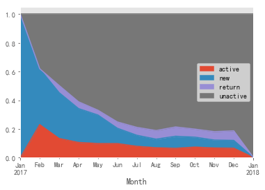
In [33]:
active_status.replace('unreg', np.nan).apply(lambda x:x.value_counts()).fillna(0).T.apply(lambda x: x/x.sum(),axis=1).plot.area()
Out[33]:
<matplotlib.axes._subplots.AxesSubplot at 0x1e991f66d30>
As can be seen from the above figure:
- New users: the proportion of new users shows an obvious downward trend, indicating that the new operation is insufficient
- Active users: the proportion reached the highest in February, followed by a slow downward trend, indicating that the consumption operation is declining
- Inactive users: inactive users show an obvious upward trend, and the loss of customers is more obvious
- Return customers: there is a slow upward trend, indicating that the recall operation is good
4. User life cycle analysis
(1) User lifecycle distribution
In [34]:
#The data samples constituting the user life cycle research need users with consumption times > = 2 times
clv = (grouped_customer[['Sales_Amount']].sum())[grouped_customer.Transaction_ID.nunique() > 1]
In [35]:
clv['lifetime'] = (grouped_customer.Date.max() - grouped_customer.Date.min())/np.timedelta64(1,'D')
In [36]:
clv.describe()
Out[36]:
| Sales_Amount | lifetime | |
|---|---|---|
| count | 11090.000000 | 11090.000000 |
| mean | 121.473811 | 116.468260 |
| std | 202.733651 | 85.985488 |
| min | 2.240000 | 0.000000 |
| 25% | 27.462500 | 42.000000 |
| 50% | 55.635000 | 96.000000 |
| 75% | 126.507500 | 190.000000 |
| max | 3985.940000 | 364.000000 |
- It can be seen from the above table that the average life cycle of users who consume more than once is 116 days, and the average consumption amount in the user's life cycle is 121.47 yuan
In [37]:
clv['lifetime'].plot.hist(bins = 50)
Out[37]:
<matplotlib.axes._subplots.AxesSubplot at 0x1e991ab1400>
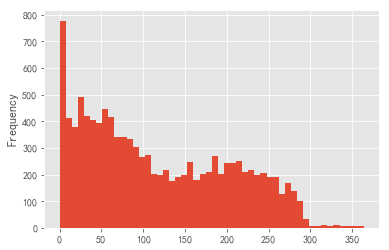
As can be seen from the above figure:
- There are many users with a life cycle of 0-90 days, indicating that customers with a short life cycle account for a high proportion and a high turnover rate within 90 days. This part of users can be used as the focus of operation to prolong the life cycle of these users;
- The life cycle is evenly distributed between 90-250, which is also the life cycle of most users, which can stimulate their consumption and increase their consumption amount in the life cycle;
- Few people have a life cycle greater than 250 days, indicating that the proportion of loyal customers with a long life cycle is not high.
(2) User life cycle value distribution
In [38]:
clv['Sales_Amount'].plot.hist(bins = 50)
Out[38]:
<matplotlib.axes._subplots.AxesSubplot at 0x1e99178d208>
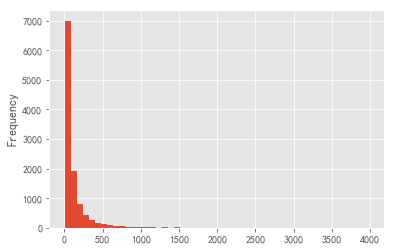
As can be seen from the above figure:
- The value of most users in the life cycle is within 500, and most of them are within 100. There are large extreme values, raising the average value, and the data skews to the right.
(3) User life cycle and its value relationship
In [39]:
plt.scatter(x='lifetime', y='Sales_Amount', data=clv)
Out[39]:
<matplotlib.collections.PathCollection at 0x1e991810518>
As can be seen from the above figure:
- There is no linear relationship between the user's life cycle and its customer value. When the life cycle is within 300 days, the value contributed by some users with longer life cycle is higher than that of users with shorter life cycle;
- When the life cycle is more than 300 days, some users contribute less value. Due to insufficient data, the results are only for reference
5. Analysis of repurchase rate and repurchase rate
(1) Repurchase rate analysis
In [40]:
#Number of users whose monthly consumption times are greater than 1
customer_month_again = grouped_month_customer.nunique().query('Transaction_ID > 1').reset_index().groupby('Month').count().Customer_ID
#Monthly consumption users
customer_month = grouped_month.Customer_ID.nunique()
#Monthly repurchase rate
(customer_month_again/customer_month).plot()
Out[40]:
<matplotlib.axes._subplots.AxesSubplot at 0x1e991788390>

- It can be seen from the above figure that the repurchase rate fluctuates around 25%, which means that 25% of users will spend many times every month; The repurchase rate decreased in the first three months, picked up in the follow-up and showed an overall upward trend. We should decide whether to further improve the repurchase rate or focus on the acquisition of new users in combination with our own business model. Due to the lack of data in the last month, the results are mainly real data.
(2) Repurchase rate analysis
In [41]:
#  1 means consumption in the first 90 days and repurchase in this month. 0 means consumption in the first 90 days and no repurchase in this month. nan means no consumption in the first 90 days
def buy_back(data):
    status = [np.nan,np.nan,np.nan]
    for i in range(3,len(data)):
        #Purchase this month
        if data[i] == 1:
            #Purchase in the first 90 days
            if (data[i-1] == 1 or data[i-2] ==1 or data[i-3] == 1):
                status.append(1)
            #Not purchased in the first 90 days
            else:
                status.append(np.nan)
        #Not purchased this month
        else:
            #Purchase in the first 90 days
            if (data[i-1] == 1 or data[i-2] ==1 or data[i-3] == 1):
                status.append(0)
            #Not purchased in the first 90 days
            else:
                status.append(np.nan)
    status = pd.Series(status, index = data.index)
    return status
In [42]:
back_status = pivoted_status.apply(buy_back, axis=1)
back_status.head()
Out[42]:
| Month | 2017-01-01 | 2017-02-01 | 2017-03-01 | 2017-04-01 | 2017-05-01 | 2017-06-01 | 2017-07-01 | 2017-08-01 | 2017-09-01 | 2017-10-01 | 2017-11-01 | 2017-12-01 | 2018-01-01 |
|---|---|---|---|---|---|---|---|---|---|---|---|---|---|
| Customer_ID | |||||||||||||
| 1 | NaN | NaN | NaN | NaN | NaN | NaN | NaN | NaN | NaN | NaN | NaN | NaN | NaN |
| 2 | NaN | NaN | NaN | 0.0 | 0.0 | 1.0 | 0.0 | 0.0 | 0.0 | NaN | NaN | NaN | NaN |
| 3 | NaN | NaN | NaN | NaN | NaN | NaN | NaN | NaN | NaN | NaN | NaN | NaN | NaN |
| 4 | NaN | NaN | NaN | NaN | NaN | NaN | NaN | 0.0 | 0.0 | 0.0 | NaN | NaN | NaN |
| 5 | NaN | NaN | NaN | 0.0 | 1.0 | 0.0 | 1.0 | 0.0 | 0.0 | 0.0 | NaN | NaN | NaN |
In [43]:
(back_status.sum()/back_status.count()).plot()
Out[43]:
<matplotlib.axes._subplots.AxesSubplot at 0x1e9952a1390>

- It can be seen from the above figure that the repurchase rate within 90 days, that is, the repeat purchase rate within 90 days is less than 10%, indicating that the store is in the user acquisition mode. However, according to the previous analysis, the acquisition of new users is on the decline. At present, the store is not healthy, and the focus should be on the acquisition of new users at the current stage,
6. Commodity Association Rule Mining
(1) Analyze hot selling goods
In [44]:
#Take out the top 10 product types
hot_category = df.groupby('SKU_Category').count().Sales_Amount.sort_values(ascending=False)[:10].reset_index()
plt.barh(hot_category.SKU_Category, hot_category.Sales_Amount)
Out[44]:
<BarContainer object of 10 artists>
In [45]:
#Proportion of best selling goods
hot_category['percent'] = hot_category.Sales_Amount.apply(lambda x:x/hot_category.Sales_Amount.sum())
plt.figure(figsize=(6,6))
plt.pie(hot_category.percent,labels=hot_category.SKU_Category,autopct='%1.2f%%')
plt.show()
In [46]:
category_list = df.groupby('Transaction_ID').SKU_Category.apply(list).values.tolist()
In [47]:
from apyori import apriori
In [48]:
min_support_value = 0.02
min_confidence_value = 0.3
result = list(apriori(transactions=category_list, min_support=min_support_value, min_confidence=min_confidence_value, min_left=0))
In [49]:
result
Out[49]:
[RelationRecord(items=frozenset({'FU5', 'LPF'}), support=0.02067035651340404, ordered_statistics=[OrderedStatistic(items_base=frozenset({'FU5'}), items_add=frozenset({'LPF'}), confidence=0.4946355900850906, lift=6.8819142262602355)]),
 RelationRecord(items=frozenset({'LPF', 'IEV'}), support=0.031152407161188583, ordered_statistics=[OrderedStatistic(items_base=frozenset({'IEV'}), items_add=frozenset({'LPF'}), confidence=0.4889589905362776, lift=6.802935131397615), OrderedStatistic(items_base=frozenset({'LPF'}), items_add=frozenset({'IEV'}), confidence=0.43342654334265435, lift=6.802935131397614)]),
 RelationRecord(items=frozenset({'OXH', 'LPF'}), support=0.020067406697381034, ordered_statistics=[OrderedStatistic(items_base=frozenset({'OXH'}), items_add=frozenset({'LPF'}), confidence=0.4810971089696071, lift=6.693551990185444)])]
From the above results:
- 'FU5' -- > 'LPF': the support is about 2.1% and the confidence is about 49.5%. It shows that the probability of purchasing these two types of goods at the same time is about 2.1%. After purchasing FU5 products, the probability of purchasing LPF products at the same time is 49.5%
- 'IEV' -- > 'LPF': the support is about 3.1% and the confidence is about 48.9%. It shows that the probability of purchasing these two types of goods at the same time is about 3.1%, and the probability of purchasing IEV type products first and LPF type products at the same time is about 48.9%
'LPF' -- > 'IEV': the support is about 3.1% and the confidence is about 43.3%. It shows that the probability of purchasing these two types of goods at the same time is about 3.1%, and the probability of purchasing LPF type products first and IEV type products at the same time is about 43.3% - 'OXH' -- > 'LPF': the support is about 2.0% and the confidence is about 48.1%. It shows that the probability of purchasing these two types of goods at the same time is about 2.0%, and the probability of purchasing IEV type products first and LPF type products at the same time is about 48.1%