Written in front: This article is some new thoughts I got after Rereading SSD (SSD: Single Shot MultiBox Detector) and fastercnn (fast r-cnn: directions real time object detection with region proposal networks), and these understandings are deeper for me.

Thanks for the basic explanation from Bubbliiiing, University of science and technology of China

NMS and soft NMS

Hard NMS

non max suppression (NMS) is a commonly used algorithm in target detection tasks. NMS can filter out the box with the largest score belonging to the same category in a certain area.

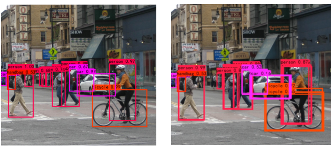
The left figure shows the results after NMS processing, and the right figure shows the results without NMS processing;

For the non maximum suppression of multi classification, it is assumed that the input shape is: [ b a t c h   s i z e , n u m   a n c h o r , 5 + n u m   c l a s s ] [batch\, size,num\, anchor,5+num\, class] [batchsize,numanchor,5+numclass], the first dimension is the number of pictures, the second dimension is the anchor of all a priori boxes, and the third dimension is the prediction results of all a priori boxes. 5 = 4 + 1, 4 represents the position of the box, and 1 represents the confidence of whether the prediction box contains objects.

The process of NMS is as follows:

• 1. Cycle all pictures;
• 2. Find out the box in the picture where the score (whether it contains the confidence of the object) is greater than the confidence threshold. The number of coincidence boxes can be greatly reduced by screening the scores before screening the coincidence boxes;
• 3. Judge the type and score of the box obtained in step 2. Take out the position of the box in the prediction result. At this time, the content in the last dimension is determined by 5 + n u m   c l a s s 5+num\, class 5+numclass becomes 4 + 1 + 2. 4 represents the position of the box, 1 represents the confidence of whether the prediction box contains an object, and 2 represents the confidence (probability) and type (from 0 to 2) of the type respectively n u m   c l a s s − 1 num\, class-1 numclass−1)；
• 4. Cycle the categories. The function of non maximum inhibition is to screen the box with the largest score of the same category (including the confidence of objects or not) in a certain area. Cycling the categories can help us carry out non maximum inhibition for each category respectively;
• 5. Sort the category from large to small according to the score;
• 6. Take out the box with the largest score each time and calculate its coincidence degree (IoU) with all other prediction frames. If the coincidence degree is too large, it will be eliminated;

Further description of step 6 is as follows:

• Take out the one with the highest score in the current category box, record it as current_box, and keep it;
• Calculate the IoU of current_box and other boxes. If the IoU is greater than the set threshold, discard these boxes;
• From the remaining box es, take out the one with the largest score, and repeat this cycle;

The implementation of IoU is as follows:

def iou(b1, b2):
    b1_x1, b1_y1, b1_x2, b1_y2 = b1[0], b1[1], b1[2], b1[3]
    b2_x1, b2_y1, b2_x2, b2_y2 = b2[:, 0], b2[:, 1], b2[:, 2], b2[:, 3]

    inter_rect_x1 = np.maximum(b1_x1, b2_x1)
    inter_rect_y1 = np.maximum(b1_y1, b2_y1)
    inter_rect_x2 = np.minimum(b1_x2, b2_x2)
    inter_rect_y2 = np.minimum(b1_y2, b2_y2)

    inter_area = np.maximum(inter_rect_x2 - inter_rect_x1, 0) * \
                 np.maximum(inter_rect_y2 - inter_rect_y1, 0)

    area_b1 = (b1_x2 - b1_x1) * (b1_y2 - b1_y1)
    area_b2 = (b2_x2 - b2_x1) * (b2_y2 - b2_y1)

    iou = inter_area / np.maximum((area_b1 + area_b2 - inter_area), 1e-6)
    return iou

NMS is implemented as follows:

import numpy as np

def non_max_suppression(boxes, num_classes, conf_thres=0.5, nms_thres=0.4):
    bs = np.shape(boxes)[0]
    # Convert the box to the form of upper left corner and lower right corner
    shape_boxes = np.zeros_like(boxes[:, :, :4])
    shape_boxes[:, :, 0] = boxes[:, :, 0] - boxes[:, :, 2] / 2
    shape_boxes[:, :, 1] = boxes[:, :, 1] - boxes[:, :, 3] / 2
    shape_boxes[:, :, 2] = boxes[:, :, 0] + boxes[:, :, 2] / 2
    shape_boxes[:, :, 3] = boxes[:, :, 1] + boxes[:, :, 3] / 2

    boxes[:, :, :4] = shape_boxes
    output = []
    # 1. Cycle through all pictures.
    for i in range(bs):
        prediction = boxes[i]
        # 2. Find the box in the picture whose score is greater than the threshold function. Filtering the score before screening the coincidence box can greatly reduce the number of boxes.
        mask = prediction[:, 4] >= conf_thres
        prediction = prediction[mask]
        if not np.shape(prediction)[0]:
            continue

        # 3. Determine the type and score of the box obtained in step 2.
        # Take out the position of the box in the prediction result and stack it.
        # At this time, the content in the last dimension changes from 5+num_classes to 4 + 1 + 2,
        # Four parameters represent the position of the box, one parameter represents whether the prediction box contains objects, and the two parameters represent the confidence and type of types respectively.
        class_conf = np.expand_dims(np.max(prediction[:, 5:5 + num_classes], 1), -1)
        class_pred = np.expand_dims(np.argmax(prediction[:, 5:5 + num_classes], 1), -1)
        detections = np.concatenate((prediction[:, :5], class_conf, class_pred), 1)
        unique_class = np.unique(detections[:, -1])

        if len(unique_class) == 0:
            continue

        best_box = []
        # 4. Cycle the species,
        # The function of non maximal inhibition is to screen out the box with the largest score belonging to the same category in a certain area,
        # Looping through classes can help us suppress each class individually.
        for c in unique_class:
            cls_mask = detections[:, -1] == c

            detection = detections[cls_mask]
            scores = detection[:, 4]
            # 5. Sort the category from large to small according to the score.
            arg_sort = np.argsort(scores)[::-1]
            detection = detection[arg_sort]
            print(detection)
            while np.shape(detection)[0] > 0:
                # 6. Take out the box with the largest score each time and calculate its coincidence degree with all other prediction frames. If the coincidence degree is too large, it will be eliminated.
                best_box.append(detection[0])
                if len(detection) == 1:
                    break
                # Calculate the IoU of the box with the highest score and the remaining box
                ious = iou(best_box[-1], detection[1:])
                # Keep the box where IoU is less than NMS threshold
                detection = detection[1:][ious < nms_thres]
        output.append(best_box)
    return np.array(output)

Soft NMS

Flexible non maximum inhibition believes that it should not be screened only through IoU. As shown in the figure, it is obvious that there are two horses in the picture (the front horse scores 0.95 and the rear horse scores 0.8), but at this time, the coincidence degree IoU of the two horses is high. At this time, if we use hard nms, the latter horse with low score will be directly eliminated.

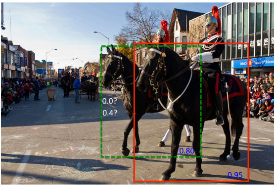
Soft NMS believes that the coincidence degree IoU and score should be considered at the same time when non maximum inhibition is carried out;

The change of Soft NMS relative to NMS is very small. For NMS, NMS directly removes the box with a high degree of coincidence with the box with the largest score. While Soft NMS takes the Gaussian index of the obtained IoU in the form of a weight, multiplies it by the original score, and then reorders it. Continue the cycle.

The implementation of Soft NMS is as follows:

def soft_non_max_suppression(boxes, num_classes, conf_thres=0.5, sigma=0.5):
    bs = np.shape(boxes)[0]
    # Convert the box to the form of upper left corner and lower right corner
    shape_boxes = np.zeros_like(boxes[:, :, :4])
    shape_boxes[:, :, 0] = boxes[:, :, 0] - boxes[:, :, 2] / 2
    shape_boxes[:, :, 1] = boxes[:, :, 1] - boxes[:, :, 3] / 2
    shape_boxes[:, :, 2] = boxes[:, :, 0] + boxes[:, :, 2] / 2
    shape_boxes[:, :, 3] = boxes[:, :, 1] + boxes[:, :, 3] / 2

    boxes[:, :, :4] = shape_boxes
    output = []
    # 1. Cycle through all pictures.
    for i in range(bs):
        prediction = boxes[i]
        # 2. Find the box in the picture whose score is greater than the threshold function. Filtering the score before screening the coincidence box can greatly reduce the number of boxes.
        mask = prediction[:, 4] >= conf_thres
        prediction = prediction[mask]
        if not np.shape(prediction)[0]:
            continue

        # 3. Determine the type and score of the box obtained in step 2.
        # Take out the position of the box in the prediction result and stack it.
        # At this time, the content in the last dimension changes from 5+num_classes to 4 + 1 + 2,
        # Four parameters represent the position of the box, one parameter represents whether the prediction box contains objects, and the two parameters represent the confidence and type of types respectively.
        class_conf = np.expand_dims(np.max(prediction[:, 5:5 + num_classes], 1), -1)
        class_pred = np.expand_dims(np.argmax(prediction[:, 5:5 + num_classes], 1), -1)
        detections = np.concatenate((prediction[:, :5], class_conf, class_pred), 1)
        unique_class = np.unique(detections[:, -1])

        if len(unique_class) == 0:
            continue

        best_box = []
        # 4. Cycle the species,
        # The function of non maximal inhibition is to screen out the box with the largest score belonging to the same category in a certain area,
        # Looping through classes can help us suppress each class individually.
        for c in unique_class:
            cls_mask = detections[:, -1] == c

            detection = detections[cls_mask]
            scores = detection[:, 4]
            # 5. Sort the category from large to small according to the score.
            arg_sort = np.argsort(scores)[::-1]
            detection = detection[arg_sort]
            print(detection)
            while np.shape(detection)[0] > 0:
                # 6. The differences between Soft NMS and NMS are as follows
                # Take out the box with the highest posterior score
                best_box.append(detection[0])
                if len(detection) == 1:
                    break
                ious = iou(best_box[-1], detection[1:])
                # The obtained IOU is multiplied by the original score after taking the Gaussian index, and then reordered
                """
                np.exp(-(ious * ious) / sigma)Equivalent to a iou Calculated weight, The value is 0-1 between
                ious The bigger, The smaller the weight value
                """
                detection[1:, 4] = np.exp(-(ious * ious) / sigma) * detection[1:, 4]
                # Operate the remaining boxes after the first box is removed from the posterior score
                detection = detection[1:]
                # Reorder according to a posteriori score (combining IoU and score)
                scores = detection[:, 4]
                arg_sort = np.argsort(scores)[::-1]
                detection = detection[arg_sort]
        output.append(best_box)
    return np.array(output)

It can be seen that Soft NMS comprehensively considers the score of a priori box and IoU, and solves the problem of horse target detection in the figure above to a certain extent.

One Stage and Two Stage

One Stage: SSD

Before SSD processes an image, it first makes the following assumptions to divide the image into grid s of different scales:

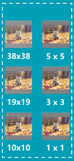
In the grid, each small block is responsible for detecting the corresponding object at that position. Obviously, dense grid is conducive to detecting small targets and sparse grid is conducive to detecting large targets;

Let's review the architecture of SSD:

When the input image is calculated on the convolution path, six feature maps of different sizes can be obtained. Pay attention to their sizes (38x38, 19x19, 10x10, 5x5, 3x3, 1x1), which exactly correspond to each point (pixel) of the feature map on the previously assumed grid It corresponds to a small block in the grid. Then, we can realize multi-scale target detection only by processing each feature map separately;

Now, there are six feature graphs to be processed in the next step. In order to distinguish from ordinary feature graphs, we call them effective feature graphs;

For each effective feature map, two operations shall be carried out at the same time:

• Once num_ Convolution of anchors x 4;
• Once num_ anchors x num_ Convolution of classes;

And num_anchors refers to the number of prior frames owned by each feature point of the feature graph. For the six feature graphs mentioned above, the number of prior frames corresponding to each feature point of each feature graph is 4, 6, 6, 6, 4 and 4 respectively.

The a priori box is initialized by us in advance:

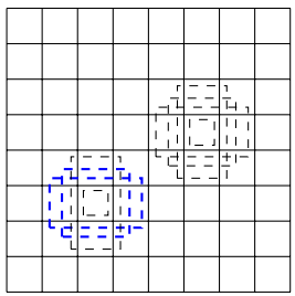
Each small block (corresponding to a feature point on the effective feature graph) is associated with several a priori boxes of different shapes. Each small block in the above figure corresponds to four a priori boxes (also known as anchor)

In order to observe the operation of one stage, review the SSD architecture. In the SSD paper, the model architecture is as follows:

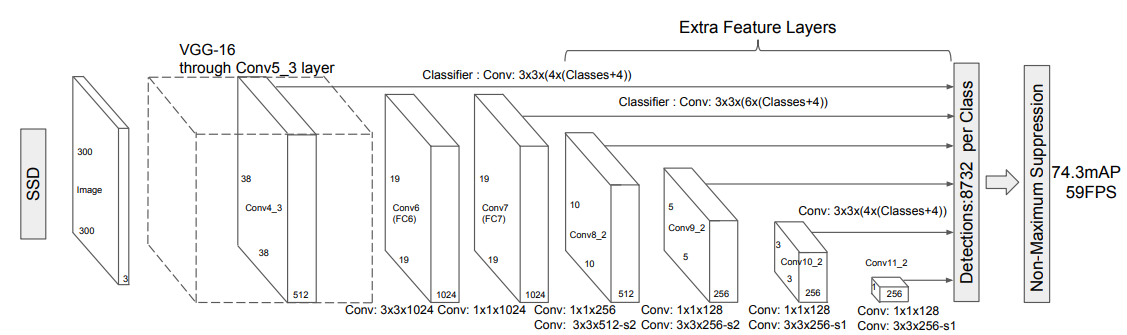
Taking the effective feature map (512x38x38) as an example, the feature map is calculated by convolution. The kernel size is 3X3, and the number of filters is 4x(Classes+4). The first number 4 represents four anchors corresponding to each feature point, and the second number 4 represents the correction information of each anchor (the offset of the coordinates in the upper left corner and the lower right corner), Classes represents the probability distribution that each anchor belongs to a class;

Equivalently, the above convolution operation can be decomposed into the following two synchronous operations (equivalent to the splitting of channels, the effect is consistent and easy to understand):

The essence of convolution is that the local fully connected network slides on the image as a kernel, so it has the property of calculating the similarity of the fully connected network, which is easy to understand for the branches of CNN classification;

Understanding of convolution networks for regression:
Input a feature map, a filter in the one-layer convolution model slides on the image, and a check of the filter corresponds to a layer of two-dimensional array in the feature map. For this two-dimensional array, the brightness in the local area represents the activation degree of a feature corresponding to this area;
On the surface, our filter operation is to perform nonlinear regression on the local area according to the characteristics of the output channel (corresponding to the current filter). In fact, it is also a kind of pattern recognition. The calculation of dot product helps us obtain the degree information of the object in the local area deviating from the center of the template object;
If we take a specific anchor analysis as an example, the convolution corresponds to four filters, which are responsible for identification respectively x 0 , y 0 , x 1 , y 1 x_{0},y_{0},x_{1},y_{1} The deviation degree of x0, y0, x1, y1} can be imagined if x 0 x_{0} x0 ， the coordinates of the upper left corner relative to the ground truth are right biased, and the network outputs a positive number to correct x 0 x_{0} x0 ， to move to the left;

Why is it so effective?
coordinate x x x can only move left and right to correct the coordinates y y y can only move up and down for correction, which can be reflected by the positive and negative of the value, which makes convolution achieve the effect of "regression", but it still belongs to the recognition of a certain pattern in essence

After obtaining the coordinate correction information and classification probability distribution of all anchors, first correct the position of each anchor. At this time, it is renamed bounding box. NMS is used as post-processing. After deleting the redundant box, the final target detection result can be output.

Two Stage: FasterRCNN

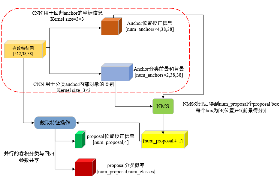
For FasterRCNN, it can be seen as a further refinement of the one stage model. FasterRCNN will also obtain the feature map through the convolution path (backbone), but the feature map is relatively dense. Similarly, each feature point is associated with a group of anchor s of different shapes, and then carry out the same convolution regression and classification operation as one satge (corresponding to the red dashed box in the figure below), but only the foreground and background (i.e. whether objects are included) are classified at this time Then, the foreground frames are corrected with the regressed position information, NMS is performed on these foreground frames, the features corresponding to the feature map in the frame are taken out, and the convolution classification and regression of these features are carried out again. At this time, the regression will be used as the further refinement of the position, and the classification is to subdivide the foreground object into various categories of the target object.

Relationship between One Stage and Two Stage

From the above description, it can be found that the feature of one stage is that the model can simultaneously calculate and output the category probability distribution of the a priori frame anchor and its position correction information, and then use NMS post-processing to obtain the target detection results;

The characteristic of two stage is that the model first calculates the category probability and location correction information of anchor like one stage, but the category probability here only distinguishes between foreground and background;
Then, the anchor containing the foreground is corrected, and then NMS is used for post-processing to obtain the proposal box. The proposal box returns to the feature map to intercept the corresponding features, and convolution regression (location refinement) and specific category classification are carried out respectively.

two stage considers the a priori conditions of foreground and background, which helps the model detect specific objects more accurately, but it also obviously increases the computational overhead.