1 pandas Library
Our general alias is pd:
import pandas as pd
pandas can not only read data from a variety of different file formats, but also have a variety of data processing functions.
1.1 using pandas to read csv files
The pandas module provides a read_ csv method, you can directly read the csv file and return a DataFrame object. DataFrame object is the core of pandas module. All tables of pandas are stored through DataFrame object, and DataFrame also provides many methods to view and modify data.
Note: to make the DataFrame object print better (in the Jupiter notebook), put the DataFrame variable at the end of the Cell to make it look better.
1.2 using pandas to read excel files
pandas also provides read_excel function to read the contents of excel file, but the use method is better than read_ csv is a little more complicated.
However, excel can have multiple sheet s, so you need multiple parameters to read different tables:
# Using read_ The excel function reads the table "sheet2" in the data.xlsx file
# And save the result in DF_ In perf variable
df_perf = pd.read_excel("data.xlsx", sheet_name="sheet2")
# Let notebook print df_perf variable
df_perf
If not specified, pandas loads the first table by default.
>>Selective reading
Sometimes, there are a lot of data in excel files, and loading all of them into Python may cause a card, and sometimes we are only interested in some columns, and it is not easy to see all of them loaded and displayed. read_excel provides the usecols parameter, which can specify which columns to load.
df_perf1 = pd.read_excel("info.xlsx", sheet_name="sheet2", usecols="A,B")
# This refers to loading excel columns a and B
1.3 using pandas to read html files
Via read_ The html function extracts the table in the html content into a list of dataframes, and determines which one we want by looking at it one by one.
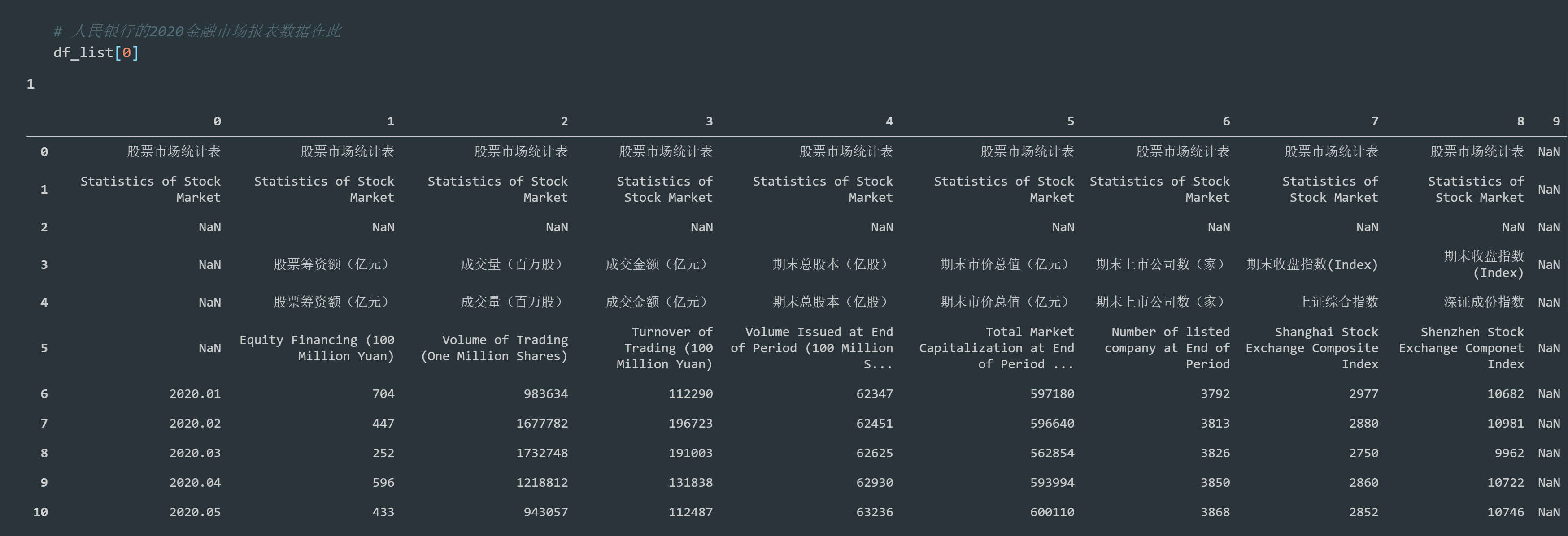
# 2020 financial market report data of the people's Bank of China
url= "http://www.pbc.gov.cn/eportal/fileDir/defaultCurSite/resource/cms/2021/01/2021011818262828764.htm"

from selenium import webdriver
brow = webdriver.Chrome()
brow.get(url)
eco_content = brow.page_source

# print(eco_content)
df_list = pd.read_html(eco_content)
print(len(df_list))

# The 2020 financial market report data of the people's Bank of China is here
df_list[0]
1.4 DataFrame object
1.4.1 key concepts
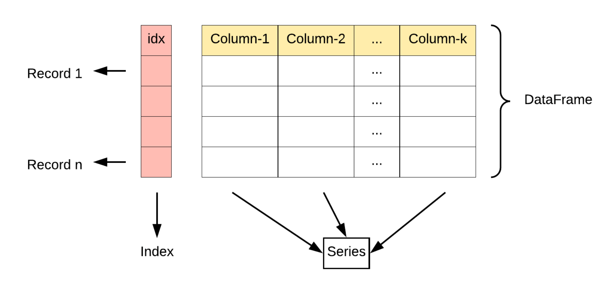
- Index: index
- Series: a data type. Series generally consists of two parts: index and values. Values is similar to a list, and index represents an index (to easily locate the data in values). In addition, series has a separate index entry, which makes it support both numerical indexes like lists and indexes like dictionaries with strings or other Python objects.
(it can be understood as a collection of lists and dictionaries [{...}, {...},...]) - DataFrame: a two-dimensional data table is actually composed of Series. A row or column of DataFrame is a Series.
1.4.2 one dimensional data Series
Create a sequence

We access two properties separately:
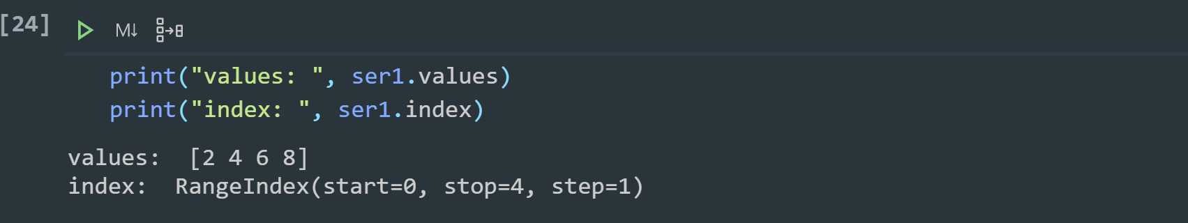
From the code output, we can see that values is actually the list value we passed in, and index is a RangeIndex object. Then we can index the values through ser1[1].
Next, try to create the Series and specify the index:

Here you can see that the corresponding index is created at the same time, and then we print the index and value:

Therefore, Series can be regarded as an advanced list or dictionary. When index is not specified, Series will generate the default location index, which is like a list. After index is specified, we can access the elements in the corresponding values through the elements in the index list, just like the key value structure of the dictionary.
1.4.3 two dimensional data table: DataFrame
The index of the Series column is the row header of the DataFrame,
The index of the row Series is the column name of the DataFrame.

(1) Construct DataFrame with Series
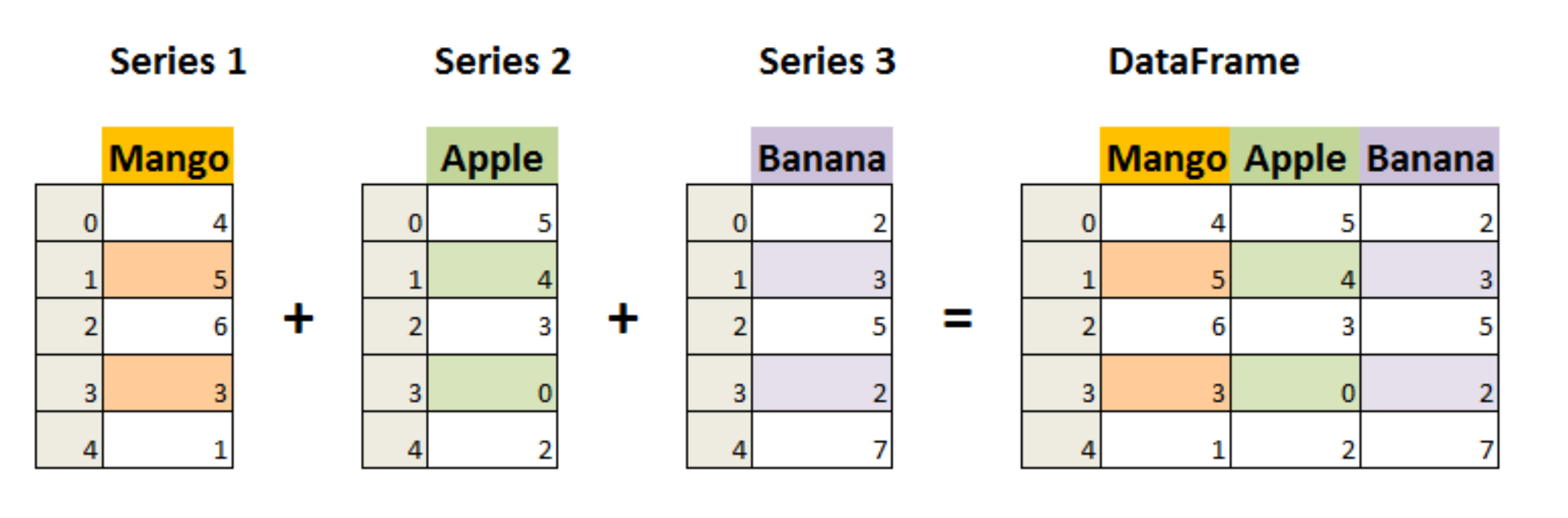
To construct this table:
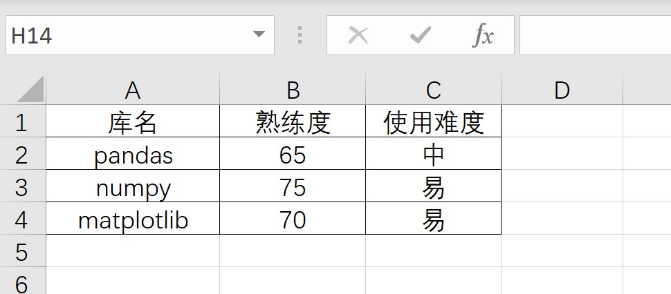
index = ['Library name', 'Proficiency', 'Use difficulty']
ser_pd = pd.Series(['pandas', 65, 'in'], index=index)
ser_np = pd.Series(['numpy', 75, 'easy'], index=index)
ser_plt = pd.Series(['matplotlib', 70, 'easy'], index=index)
df = pd.DataFrame([ser_pd, ser_np, ser_plt])
df

In addition to using Series, we can also create DataFrame objects with lists, dictionaries, numpy's ndarray objects, etc. you can refer to< Rookie tutorial: Pandas data structure - DataFrame>.
(2) Add rows and columns
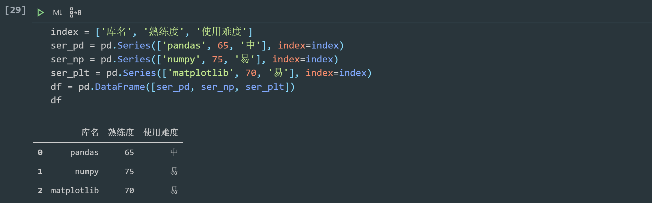
Using the append method, you can add rows to the DataFrame object:
# We add a row of data
ser_torch = pd.Series(['pytorch', 55, 'hard'], index=index)
# Setting ignore_index means that the DataFrame automatically generates row indexes
# After calling append, a new DataFrame will be returned, and we will save it back to the original variable
df = df.append(ser_torch, ignore_index= True)
# View the added DataFrame
df

Adding columns is easier:
# Assign the newly added Series to the column Series corresponding to the new column name in the DataFrame
df["Assessment results"] = pd.Series(["qualified", "excellent", "qualified", "unqualified"])
# Print
df

# Of course, you can add a value uniformly
df["Assessment results"] = "qualified"
# Print
df
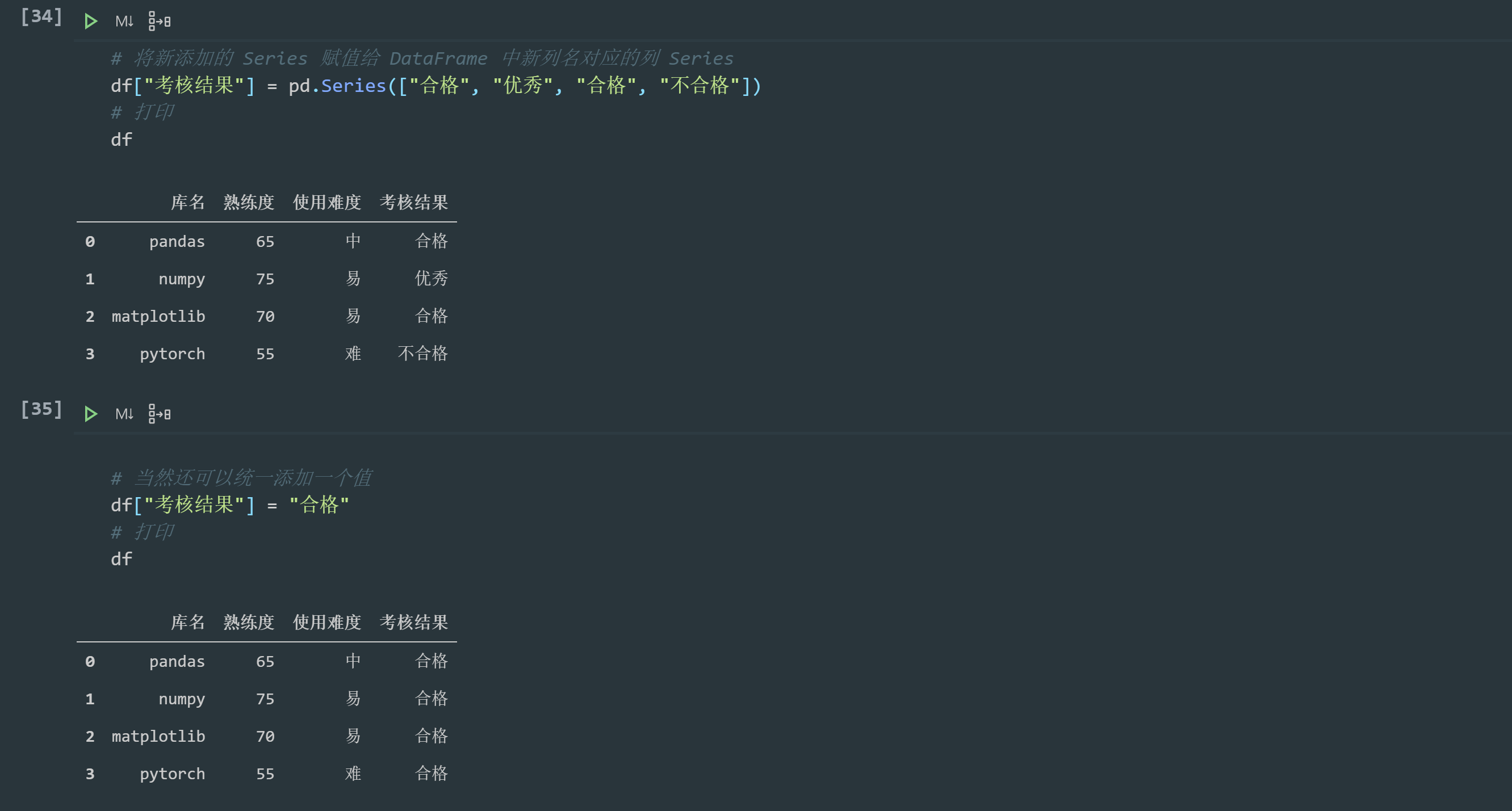
When we assign a value to the column Series corresponding to a column name in the DataFrame, when the column name does not exist, the corresponding column will be created, and when the column name exists, the value of the original column will be modified. Therefore, we can not only create new columns, but also modify existing columns.
(3) Delete rows and columns
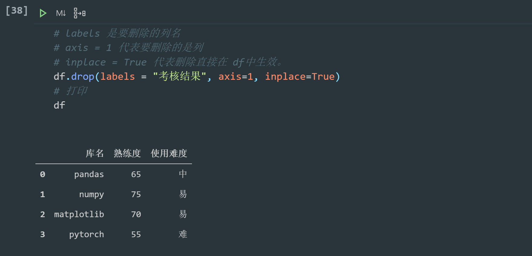
DataFrame provides a drop method to delete a row or column.
Delete column:
# labels is the name of the column to delete
# axis = 1 means the column to be deleted
# inplace = True means that the deletion takes effect directly in df.
df.drop(labels = "Assessment results", axis=1, inplace= True)
# Print
df
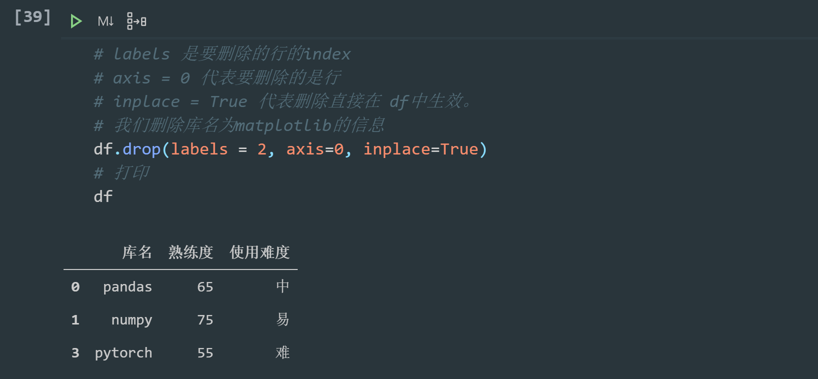
Delete row:
# labels is the index of the row to be deleted
# axis = 0 means the row to be deleted
# inplace = True means that the deletion takes effect directly in df.
# We delete the information of the library named matplotlib
df.drop(labels = 2, axis=0, inplace=True)
# Print
df
(4) Viewing and modifying a single cell

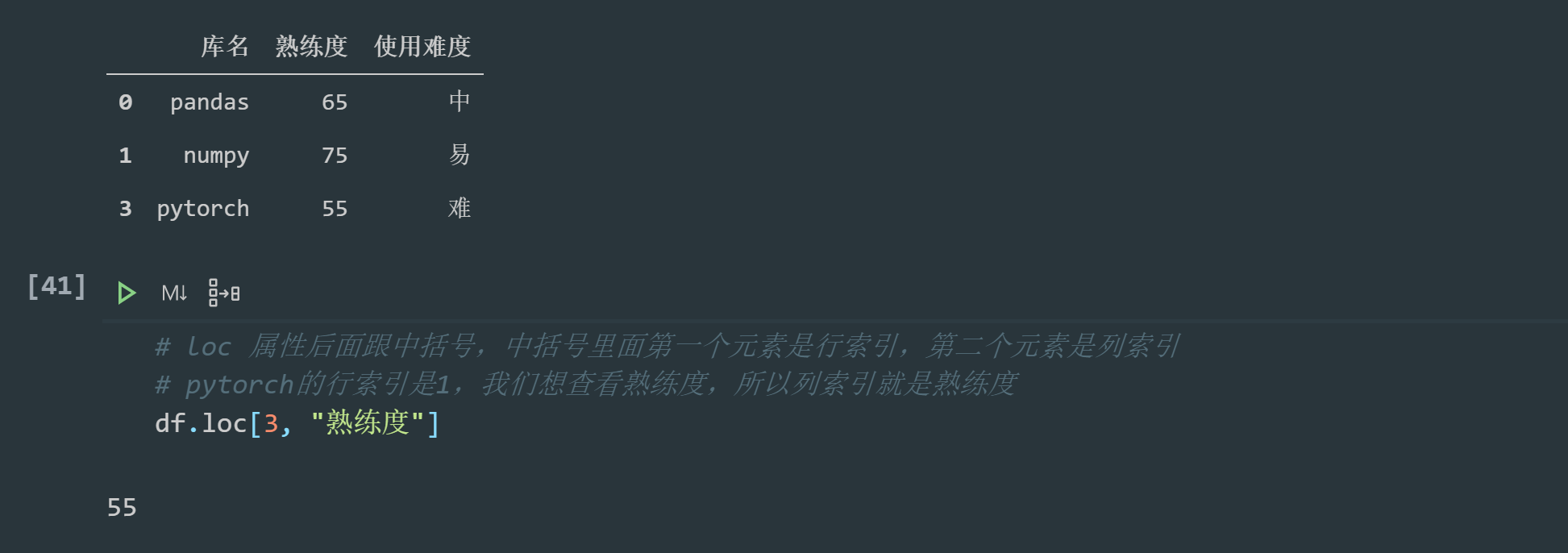
The recommended way to view and modify a single cell is to use the loc property of DataFrame, which can specify the location to the cell in one step. Suppose we need to check the proficiency of the third-party library pytorch:
# The loc attribute is followed by square brackets. The first element in the square brackets is the row index and the second element is the column index
# The row index of pytorch is 1. We want to check the proficiency, so the column index is the proficiency
df.loc[3, "Proficiency"]
Then we can modify the proficiency by assigning a value directly:
df.loc[3, "Proficiency"] = 65
(5) Sorting of DataFrame
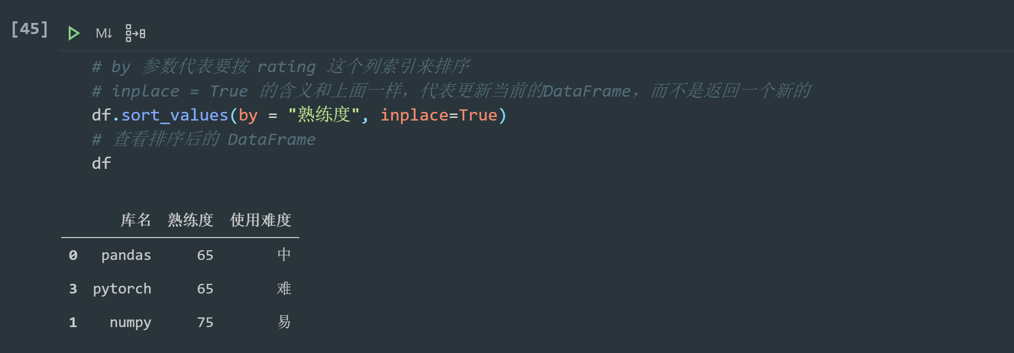
DataFrame provides sort_values method to realize sorting. For example, we want to sort the third-party library according to proficiency:
# The by parameter indicates that you want to sort by the column index of rating
# The meaning of inplace = True is the same as above. It means to update the current DataFrame instead of returning a new one
df.sort_values(by = "Proficiency", inplace=True)
# View sorted DataFrame
df
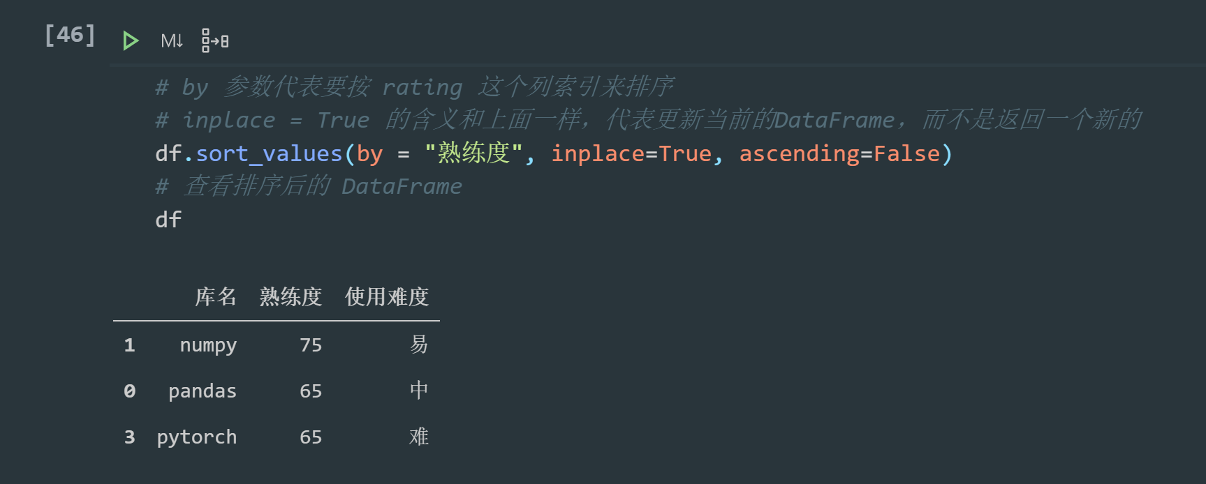
The default is ascending sorting. Descending sorting needs to be set to False:
# The by parameter indicates that you want to sort by the column index of rating
# The meaning of inplace = True is the same as above. It means to update the current DataFrame instead of returning a new one
df.sort_values(by = "Proficiency", inplace=True, ascending=False)
# View sorted DataFrame
df
It can be found from here that we deleted a row before, resulting in the loss of row 2, but it should not affect the sequence. Therefore, the digital index of Series can be discontinuous, which is also an important difference from the list.
(6) Take the head and tail and calculate the number of rows and columns
Simple operation, no demonstration is required, and it is very effective for more data.
# The head function returns the first n records of the DataFrame. N is the value specified by the function parameter
# Here we specify 10 lines
df.head(10)

# The tail function returns n records at the end of the DataFrame. N is the parameter of the function
# Here we specify 10 lines
df.tail(20)

# The shape attribute returns a tuple. The first element is the number of rows and the second element is the number of columns
shape = df.shape
# Print rows and columns
print("Number of rows:", shape[0])
print("Number of columns:", shape[1])
1.5 slicing and data query loc and iloc
1.5.1 slicing
Brackets [] are the most basic indexer in pandas, similar to slicing in python.
DataFrame and Series also support []. The specific behaviors are:
1. Use [] for Series to return the element corresponding to the index;
2. Use [] for DataFrame to return the column whose column name is equal to the index in the form of Series.
# Get library name
ser_name = df["Library name"]
print(type(ser_name))
print(ser_name)

print("----------------------")
# We can also select multiple pieces of data, return or Series
ser_name_1 = ser_name[[0,2]]
print(type(ser_name_1))
print(ser_name_1)
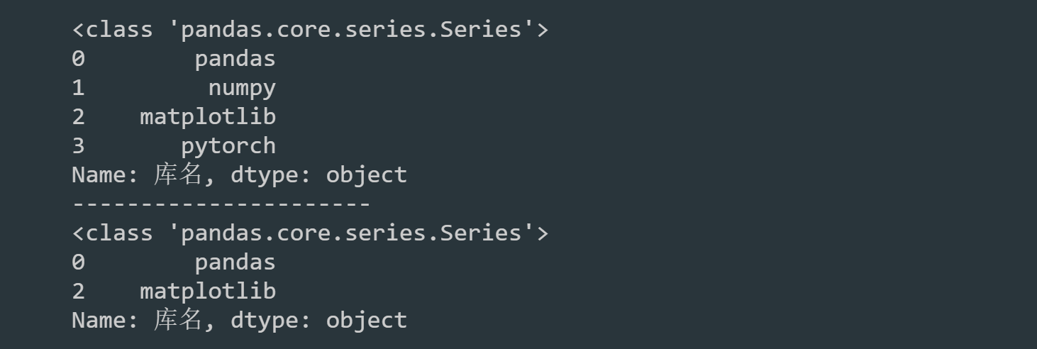
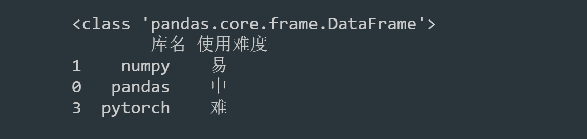
# Get new DataFrame
df_new = df[["Library name", "Use difficulty"]]
print(type(df_new))
print(df_new)
==Application of slice==

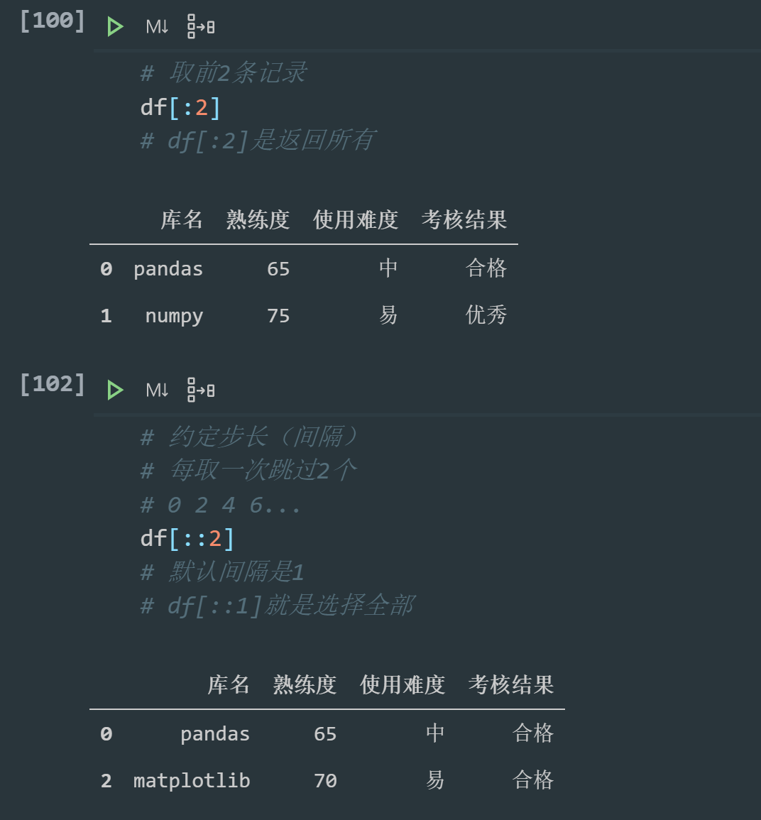
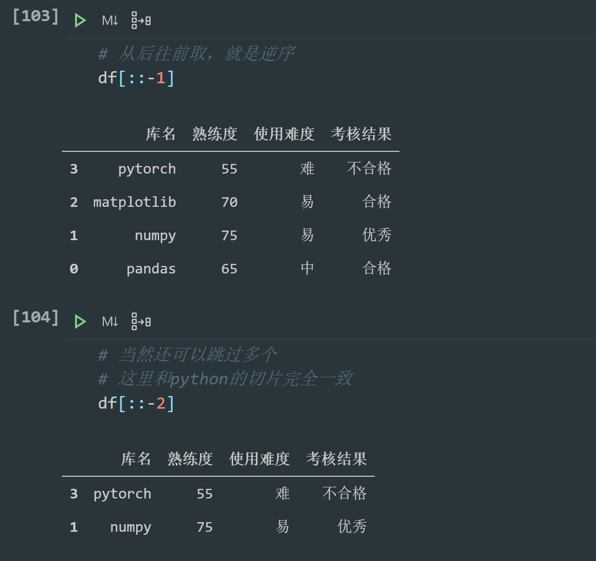
This is similar to python's slicing, so I won't go into detail. For details about python's basic data types, see the< In depth study of four important data structures in Python>.
1.5.2 data query loc and iloc
Looking up elements with slices is very clumsy, so pandas provides a set of very powerful data query methods in addition to [] indexer: loc and iloc.
pandas provides a special method for indexing DataFrame, that is, using the ix method for indexing. However, ix has been abandoned in the latest version. If you use tags, you'd better use the loc method. If you use subscripts, you'd better use the iloc method.
(1)loc
# basic form
df.loc[Row index name, Column index name]
The [] indexer of loc object supports the ability of [] indexers of all dataframes, that is, the row index part and column index part of loc object can use multiple indexes and range selection syntax respectively.

(2)iloc
The usage of iloc is very similar to loc, except that iloc only supports incoming integer indexes.
loc is the name of the row index and column index to be passed in, while iloc needs to pass in numbers such as the row and column. The basic usage is as follows:
df.iloc[What line, Which column]
(3) Condition query
df.loc[Conditional expression, Column index name]
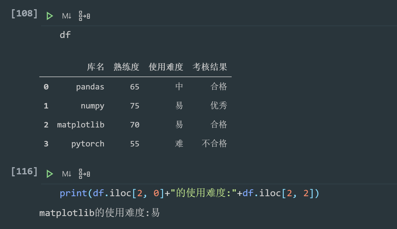
Use example:

1.6 data cleaning
1.6.1 treatment of missing values
When we load data from CSV files or other data sources into the DataFrame, we often encounter that the data of some cells is missing. When we print out the DataFrame, the missing part will be displayed as NaN, None, or NaT (depending on the data type of the cell), which is called the missing value.
We create a table with missing data: