In RNA SEQ, principal component analysis (PCA) is one of the most common types of multivariate data analysis. This issue mainly introduces how to analyze using the existing expression difference data. Don't worry, see below.
1. Preface
1. Relevant background
In RNA SEQ, principal component analysis (PCA) is one of the most common types of multivariate data analysis. After quantifying gene expression, we obtain the expression value information of all genes in each sample. Then we usually expect to compare the overall similarity or difference of gene expression values between samples. There are thousands of genes, so we can't compare the expression of each gene. At this time, we need to use the "dimension reduction" algorithm, so PCA analysis is useful. PCA tries to reduce the N-dimensional (N = number of genes) expression matrix to the form of only a few principal components, which can represent the overall expression pattern of all genes, and then describe the sample differences.
2. Data dimensionality reduction
Dimensionality reduction is a preprocessing method for high-dimensional feature data. Dimensionality reduction is to preserve the most important features of high-dimensional data and remove noise and unimportant features, so as to improve the speed of data processing. In practical production and application, dimensionality reduction within a certain range of information loss can save us a lot of time and cost. Dimensionality reduction has also become a widely used data preprocessing method.
Dimensionality reduction has the following advantages:
-
Make data sets easier to use.
-
Reduce the computational overhead of the algorithm.
-
Remove noise.
-
Make the results easy to understand.
PCA(Principal Component Analysis), that is, principal component analysis method, is one of the most widely used data dimensionality reduction algorithms. The main idea of PCA is to map n-dimensional features to k-dimension, which is a new orthogonal feature, also known as the main component. It is a k-dimensional feature reconstructed from the original n-dimensional features. The job of PCA is to find a set of mutually orthogonal coordinate axes from the original space. The selection of new coordinate axes is closely related to the data itself. Among them, the first new coordinate axis selection is the direction with the largest variance in the original data, the second new coordinate axis selection is the one with the largest variance in the plane orthogonal to the first coordinate axis, and the third axis is the one with the largest variance in the plane orthogonal to the first and second axes. By analogy, n such coordinate axes can be obtained. Through the new coordinate axes obtained in this way, we find that most of the variance is contained in the first k coordinate axes, and the variance of the latter coordinate axes is almost 0. Therefore, we can ignore the remaining coordinate axes and only keep the first k coordinate axes containing most of the variance. In fact, this is equivalent to retaining only the dimension features that contain most of the variance, while ignoring the feature dimensions that contain almost zero variance, so as to reduce the dimension of data features. There are many dimensionality reduction algorithms, such as singular value decomposition (SVD), principal component analysis (PCA), factor analysis (FA), independent component analysis (ICA).
2. Example analysis
We still use the data set of TCGA-COAD for data reading. We mentioned the reading of expression data and the acquisition of clinical information grouping in the previous period. We use the differential expression results calculated by edgeR software package and combine the original Count data, as follows:
1. Data reading
The results of saving the final expression difference before can be read directly. Here we compare the expression difference between cancer and adjacent cancer. The data are as follows:
group<-read.table("DEG-group.xls",sep="\t",check.names=F,header = T)
DEG=read.table("DEG-resdata.xls",sep="\t",check.names=F,header = T)

PCAmat<-DEG[,8:ncol(DEG)]
rownames(PCAmat)=DEG[,1]
PCAmat[1:5,1:3]


##                 TCGA-3L-AA1B-01A-11R-A37K-07
## ENSG00000142959                           20
## ENSG00000163815                          175
## ENSG00000107611                           49
## ENSG00000162461                           55
## ENSG00000163959                          153
##                 TCGA-4N-A93T-01A-11R-A37K-07
## ENSG00000142959                           15
## ENSG00000163815                          108
## ENSG00000107611                           13
## ENSG00000162461                           89
## ENSG00000163959                          259
##                 TCGA-4T-AA8H-01A-11R-A41B-07
## ENSG00000142959                           49
## ENSG00000163815                           59
## ENSG00000107611                            6
## ENSG00000162461                           48
## ENSG00000163959                          102
Transpose the gene expression value matrix to list the behavior samples as genes, as follows:
PCAmat_t<-t(PCAmat)
PCAmat_t[1:5,1:3]


##                              ENSG00000142959 ENSG00000163815
## TCGA-3L-AA1B-01A-11R-A37K-07              20             175
## TCGA-4N-A93T-01A-11R-A37K-07              15             108
## TCGA-4T-AA8H-01A-11R-A41B-07              49              59
## TCGA-5M-AAT4-01A-11R-A41B-07              16              60
## TCGA-5M-AAT5-01A-21R-A41B-07              24              60
##                              ENSG00000107611
## TCGA-3L-AA1B-01A-11R-A37K-07              49
## TCGA-4N-A93T-01A-11R-A37K-07              13
## TCGA-4T-AA8H-01A-11R-A41B-07               6
## TCGA-5M-AAT4-01A-11R-A41B-07              24
## TCGA-5M-AAT5-01A-21R-A41B-07              10
2. PCA {FactoMineR}
The software package FactoMineR is installed and loaded as follows:
if(!require(FactoMineR)){
  install.packages("FactoMineR")
}

library(FactoMineR)
The method proposed in this FactoMineR is an exploratory multivariate method, such as principal component analysis, correspondence analysis or clustering. Through this package, we realize PCA analysis, as follows:
#############PCA {FactoMineR}
library(ggplot2)
library(ggrepel)
#PCA analysis of gene expression values in samples
gene.pca <- PCA(PCAmat_t, ncp = 2, scale.unit = TRUE, graph = FALSE)
The results are processed as follows:
#Extract the coordinates of the sample in the first two axes of PCA
pca_sample <- data.frame(gene.pca$ind$coord[ ,1:2])
pca_sample$Sample=row.names(pca_sample)
#Extract the contribution of the first two axes of PCA
pca_eig1 <- round(gene.pca$eig[1,2], 2)
pca_eig2 <- round(gene.pca$eig[2,2],2 )
pca_sample <- merge(pca_sample, group,by="Sample")
head(pca_sample)


##                         Sample      Dim.1       Dim.2 Group
## 1 TCGA-3L-AA1B-01A-11R-A37K-07  1.1786551  -0.7589326    TP
## 2 TCGA-4N-A93T-01A-11R-A37K-07 -1.9561110  -5.4213738    TP
## 3 TCGA-4T-AA8H-01A-11R-A41B-07 -5.1936884  -7.9477300    TP
## 4 TCGA-5M-AAT4-01A-11R-A41B-07  1.7605422 -11.8875367    TP
## 5 TCGA-5M-AAT5-01A-21R-A41B-07  0.9007755 -10.0044126    TP
## 6 TCGA-5M-AAT6-01A-11R-A41B-07 -1.8586282  -3.0063580    TP
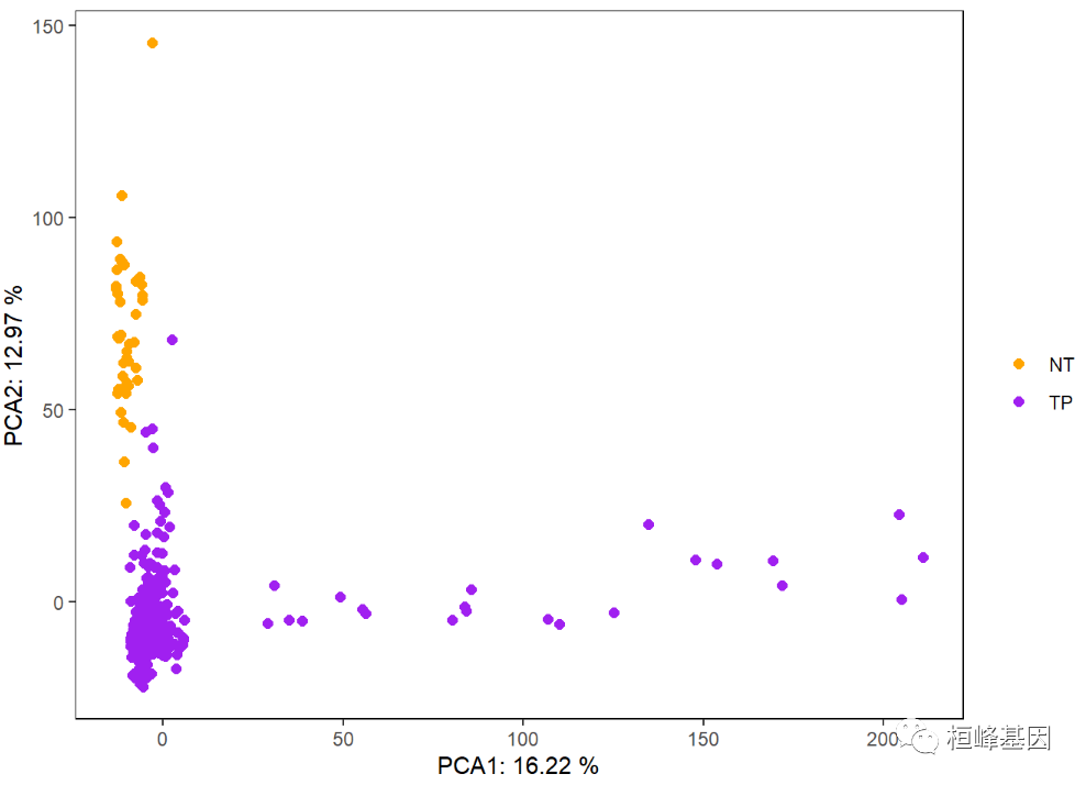
Using ggplot2 to draw a two-dimensional scatter diagram, we can see that the two groups of cancer and adjacent cancer can be basically separated. Here we choose genes with large differences, which are related, as follows:
library(ggplot2)
p <- ggplot(data = pca_sample, aes(x = Dim.1, y = Dim.2)) +
  geom_point(aes(color = Group), size = 2) +  #Draw a two-dimensional scatter diagram according to the sample coordinates
  scale_color_manual(values = c('orange', 'purple')) +  #Custom color
  theme(panel.grid = element_blank(), panel.background = element_rect(color = 'black', fill = 'transparent'),
        legend.key = element_rect(fill = 'transparent')) +  #Remove background and gridlines
  labs(x =  paste('PCA1:', pca_eig1, '%'), y = paste('PCA2:', pca_eig2, '%'), color = '')  #Add PCA axis contribution to axis title

p
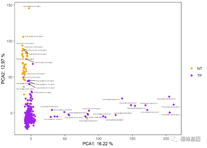
Sometimes it is also necessary to identify the sample name, which is completed by using the expansion package ggrepl of ggplot2, as follows:
library(ggrepel)
p <- p +
  geom_text_repel(aes(label = Sample), size = 1, show.legend = FALSE,
                  box.padding = unit(0.2, 'lines'))

p
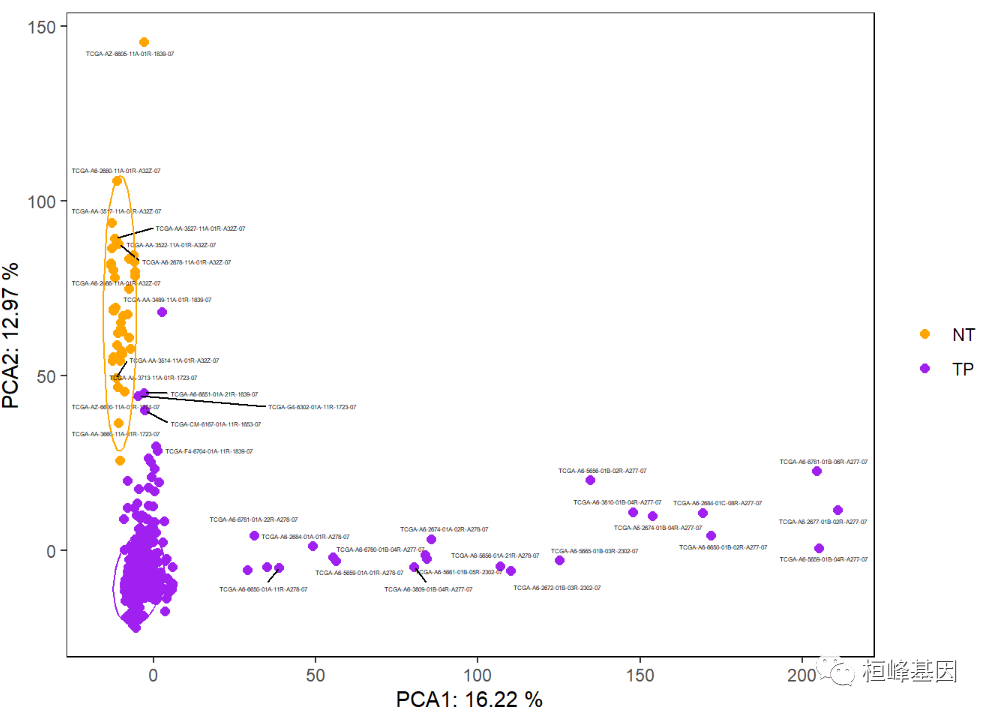
The addition of 95% confidence ellipse can be used to represent object classification, but it can only be used when the number of samples in each group is greater than 5. There are many samples here, just as an example, as follows:
p + stat_ellipse(aes(color = Group), level = 0.95, show.legend = FALSE)
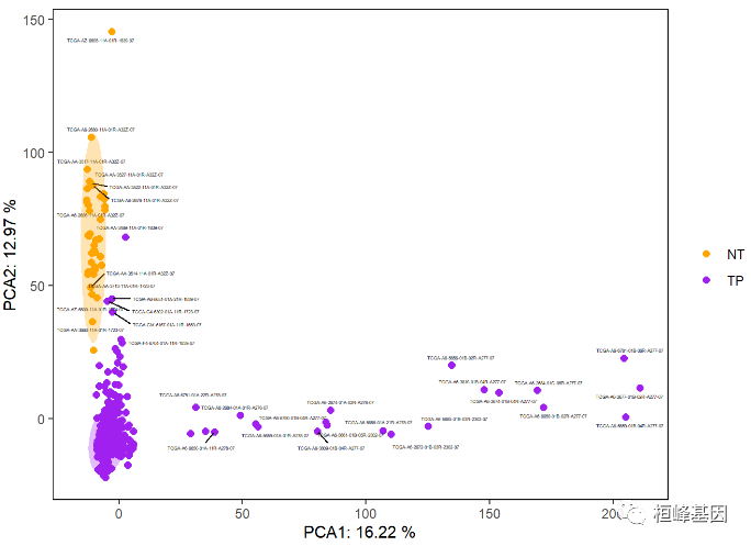
Add a shaded area as follows:
p + stat_ellipse(aes(fill = Group), geom = 'polygon', level = 0.95, alpha = 0.3, show.legend = FALSE) +
  scale_fill_manual(values = c('orange', 'purple'))
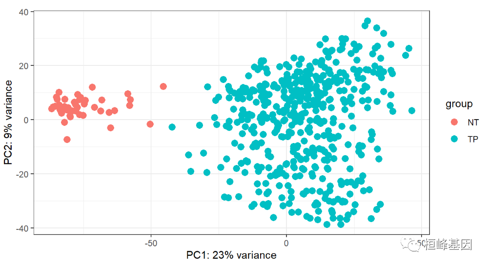
3. plotPCA {DESeq2}
When the data we use is the expression amount, we can first use the built-in function plotPCA in DESeq2 software package to draw the principal component analysis diagram, which is very convenient. Of course, we use the differentially expressed genes selected by differential expression here, which can better distinguish cancer and adjacent tissues in principal component analysis.
First, you need to construct dds objects as follows:
#####plotPCA {DESeq2}
library(DESeq2)
condition<-factor(group$Group)
dds <- DESeqDataSetFromMatrix(PCAmat,
                              DataFrame(condition),
                              design= ~ condition )
dds


## class: DESeqDataSet
## dim: 4128 519
## metadata(1): version
## assays(1): counts
## rownames(4128): ENSG00000142959 ENSG00000163815 ...
##   ENSG00000230184 ENSG00000244217
## rowData names(0):
## colnames(519): TCGA-3L-AA1B-01A-11R-A37K-07
##   TCGA-4N-A93T-01A-11R-A37K-07 ... TCGA-AZ-6605-11A-01R-1839-07
##   TCGA-F4-6704-11A-01R-1839-07
## colData names(1): condition
The data shall be standardized as follows:
rld <- vst(dds)   #DEseq2 standardizes data with its own methods`
exprSet_new=assay(rld)   #Extract DEseq2 standardized data
str(exprSet_new)


##  num [1:4128, 1:519] 3.87 6.69 4.96 5.11 6.5 ...
##  - attr(*, "dimnames")=List of 2
##   ..$ : chr [1:4128] "ENSG00000142959" "ENSG00000163815" "ENSG00000107611" "ENSG00000162461" ...
##   ..$ : chr [1:519] "TCGA-3L-AA1B-01A-11R-A37K-07" "TCGA-4N-A93T-01A-11R-A37K-07" "TCGA-4T-AA8H-01A-11R-A41B-07" "TCGA-5M-AAT4-01A-11R-A41B-07" ...
The main program draws PCA graphics as follows:
plotPCA(rld, intgroup=c('condition'))+
  theme_bw()
How's it going? Do you understand? It doesn't matter if you don't understand it. There will be a video tutorial in the next issue. You can also ask me for help to ensure your satisfaction!
Pay attention to the official account, do not go away.

References:
-
Le, S., Josse, J. & Husson, F. (2008). FactoMineR: An R Package for Multivariate Analysis. Journal of Statistical Software. 25(1). pp. 1-18.
-
Robinson MD, McCarthy DJ, Smyth GK. edgeR: a Bioconductor package for differential expression analysis of digital gene expression data. Bioinformatics. 2010;26(1):139-140.
-
Agarwal A, Koppstein D, Rozowsky J, et al. Comparison and calibration of transcriptome data from RNA-Seq and tiling arrays. BMC Genomics. 2010;11:383.
-
Love MI, Huber W, Anders S. Moderated estimation of fold change and dispersion for RNA-seq data with DESeq2. Genome Biol. 2014;15(12):550.
Huanfeng gene
Bioinformatics analysis, SCI article writing and bioinformatics basic knowledge learning: R language learning, perl basic programming, linux system commands, Python meet you better
43 original content
Official account: Huan Feng gene