1, Linear neural network

(1) Linear regression

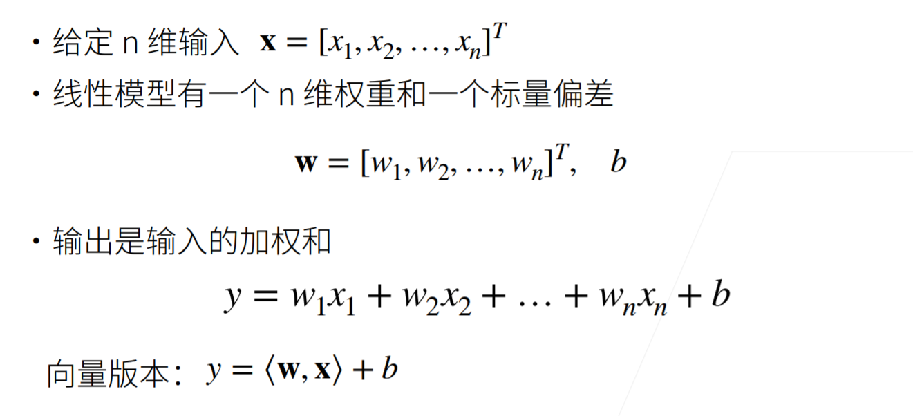
1. Linear model

The linear model is regarded as a single-layer neural network.

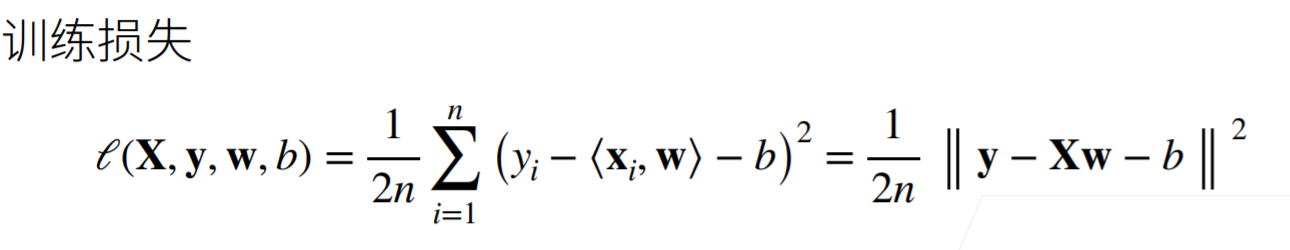
2. Loss function

The loss function can quantify the difference between the actual value and the predicted value of the target.

  3. Analytical solution

 

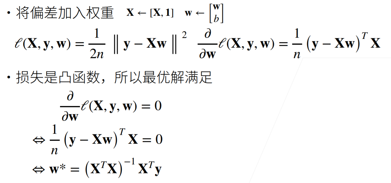
  4. Optimization method: small batch gradient descent algorithm

For the case without analytical solution, the gradient descent reduces the error by continuously updating the parameters in the decreasing direction of the loss function. Calculate the derivative (gradient) of the loss function with respect to the model parameters. But in practice, the execution may be very slow: because we have to traverse the entire data set before each parameter update. Therefore, we usually take a small batch of samples at random every time we need to calculate the update. This variant is called small batch random gradient descent, and the batch size is b.

  (2) Implementation of linear regression

1. Generate dataset

def synthetic_data(w, b, num_examples):  #@save
    """generate y = Xw + b + Noise."""
    X = torch.normal(0, 1, (num_examples, len(w)))
    y = torch.matmul(X, w) + b
    y += torch.normal(0, 0.01, y.shape)
    return X, y.reshape((-1, 1))

true_w = torch.tensor([2, -3.4])
true_b = 4.2
features, labels = synthetic_data(true_w, true_b, 1000)

2. Read dataset

Disrupt samples in the data set and obtain data in small batches. We define a data_iter function, which receives batch size, characteristic matrix and label vector as input, and generates batch size_ Small batch size. Each small batch contains a set of features and labels.

def data_iter(batch_size, features, labels):
    num_examples = len(features)
    indices = list(range(num_examples))
    # These samples are read randomly without a specific order
    random.shuffle(indices)
    for i in range(0, num_examples, batch_size):
        batch_indices = torch.tensor(
            indices[i: min(i + batch_size, num_examples)])
        yield features[batch_indices], labels[batch_indices]

3. Initialize model parameters

The weight is initialized by sampling random numbers from the normal distribution with mean value of 0 and standard deviation of 0.01, and the offset is initialized to 0.

w = torch.normal(0, 0.01, size=(2,1), requires_grad=True)
b = torch.zeros(1, requires_grad=True)

4. Define model

def linreg(X, w, b):  #@save
    """Linear regression model."""
    return torch.matmul(X, w) + b

5. Define loss function

Here we use the square loss function. In the implementation, we need to convert the shape of the real value y into and the predicted value y_hat has the same shape.

def squared_loss(y_hat, y):  #@save
    """Mean square loss."""
    return (y_hat - y.reshape(y_hat.shape)) ** 2 / 2

6. Define optimization algorithm

This function accepts the set of model parameters, learning rate and batch size as inputs. The size of each update step is determined by the learning rate lr. Because the loss we calculate is the sum of a batch of samples, we use batch_size to normalize the step size, so that the step size does not depend on our choice of batch size.

def sgd(params, lr, batch_size):  #@save
    """Small batch random gradient descent."""
    with torch.no_grad():
        for param in params:
            param -= lr * param.grad / batch_size
            param.grad.zero_()

7. Training

Number of iteration cycles num_epochs and learning rate lr are both super parameters. Setting super parameters is very difficult and needs to be adjusted through repeated experiments.  

lr = 0.03
num_epochs = 3
net = linreg
loss = squared_loss

for epoch in range(num_epochs):
    for X, y in data_iter(batch_size, features, labels):
        l = loss(net(X, w, b), y)  # `Small batch loss of X 'and' y '
        # Because the ` L 'shape is (` batch_size`, 1), not a scalar` All elements in l ` are added together,
        # And calculate the gradient about [` w`, `b `]
        l.sum().backward()
        sgd([w, b], lr, batch_size)  # Update the parameter with the gradient of the parameter
    with torch.no_grad():
        train_l = loss(net(features, w, b), labels)
        print(f'epoch {epoch + 1}, loss {float(train_l.mean()):f}')

(3) Simple implementation of linear regression

A deep learning framework is used to concisely implement the linear regression model in (2).

1. Generate dataset

import numpy as np
import torch
from torch.utils import data
from d2l import torch as d2l


true_w = torch.tensor([2, -3.4])
true_b = 4.2
features, labels = d2l.synthetic_data(true_w, true_b, 1000)

2. Read dataset

We can call the existing API in the framework to read the data. We pass features and labels as API parameters, and specify batch when instantiating the data iterator object_ size. In addition, the Boolean value is_train indicates whether you want the data iterator object to scramble the data in each iteration cycle.

def load_array(data_arrays, batch_size, is_train=True):  #@save
    """Construct a PyTorch Data iterator."""
    dataset = data.TensorDataset(*data_arrays)
    return data.DataLoader(dataset, batch_size, shuffle=is_train)

batch_size = 10
data_iter = load_array((features, labels), batch_size)

3. Define model

In PyTorch, the full connection layer is defined in the Linear class. It is worth noting that we pass two parameters to nn.Linear. The first specifies the input feature shape, i.e. 2, and the second specifies the output feature shape. The output feature shape is a single scalar, so it is 1.

# `nn ` is the abbreviation of neural network
from torch import nn

net = nn.Sequential(nn.Linear(2, 1))

4. Initialize model parameters

Just as we specify the input and output dimensions when constructing nn.Linear. Now let's access the parameters directly to set the initial value. We select the first layer in the network through net[0], and then use the weight.data and bias.data methods to access the parameters. Then use the replacement method normal_ And fill_ To override parameter values. Here, we specify that each weight parameter should be randomly sampled from a normal distribution with a mean of 0 and a standard deviation of 0.01, and the bias parameter will be initialized to zero.

net[0].weight.data.normal_(0, 0.01)
net[0].bias.data.fill_(0)

5. Define loss function

The mselos class, also known as the square L2 norm, is used to calculate the mean square error. By default, it returns the average of all sample losses.

loss = nn.MSELoss()

6. Define optimization algorithm

The small batch random gradient descent algorithm is a standard tool for optimizing neural networks. PyTorch implements many variants of the algorithm in optim module. When we instantiate the SGD instance, we need to specify the optimized parameters (which can be obtained from our model through net.parameters()) and the super parameter dictionary required by the optimization algorithm. Small batch random gradient descent only needs to set lr value, which is set to 0.03 here.

trainer = torch.optim.SGD(net.parameters(), lr=0.03)

7. Training

In each iteration cycle, we will completely traverse the train_data and constantly obtain a small batch of input and corresponding labels. For each small batch, we will carry out the following steps:

• The prediction is generated by calling net(X) and the loss l (forward propagation) is calculated.

• The gradient is calculated by back propagation.

• Update model parameters by calling the optimizer.

• num_epochs = 3
  for epoch in range(num_epochs):
      for X, y in data_iter:
          l = loss(net(X) ,y)
          trainer.zero_grad()
          l.backward()
          trainer.step()
      l = loss(net(features), labels)
      print(f'epoch {epoch + 1}, loss {l:f}')

(4) Softmax regression

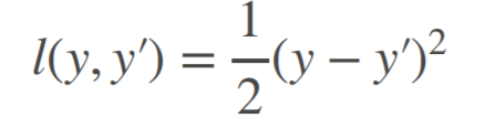
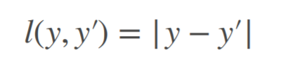
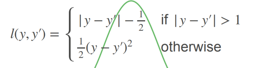
  Common loss function:

(1)L2 Loss                   (2)L1 Loss                        (3)Huber's Robust Loss

(5) Image classification dataset

%matplotlib inline
import torch
import torchvision
from torch.utils import data
from torchvision import transforms
from d2l import torch as d2l

d2l.use_svg_display()

1. Read dataset

The fashion MNIST dataset can be downloaded and read into memory through the built-in functions in the framework.

# The image data is transformed from PIL type to 32-bit floating-point format through ToTensor instance
# Divide by 255 so that the values of all pixels are between 0 and 1
trans = transforms.ToTensor()
mnist_train = torchvision.datasets.FashionMNIST(
    root="../data", train=True, transform=trans, download=True)
mnist_test = torchvision.datasets.FashionMNIST(
    root="../data", train=False, transform=trans, download=True)

Fashion MNIST contains 10 categories, each of which includes 6000 training data and 1000 test data. The following function is used to convert between a numeric label index and its text name.

def get_fashion_mnist_labels(labels):  #@save
    """return Fashion-MNIST The text label of the dataset."""
    text_labels = ['t-shirt', 'trouser', 'pullover', 'dress', 'coat',
                   'sandal', 'shirt', 'sneaker', 'bag', 'ankle boot']
    return [text_labels[int(i)] for i in labels]

2. Read small batch

Using the built-in data iterator, the data loader will read a small batch of data each time in each iteration_ size. We also randomly scrambled all samples in the training data iterator.

batch_size = 256

def get_dataloader_workers():  #@save
    """Four processes are used to read data."""
    return 4

train_iter = data.DataLoader(mnist_train, batch_size, shuffle=True,
                             num_workers=get_dataloader_workers())

Take a look at the time it takes to read the training data.

timer = d2l.Timer()
for X, y in train_iter:
    continue
f'{timer.stop():.2f} sec'

3. Consolidate all components

We define load_data_fashion_mnist function, which is used to obtain and read the fashion MNIST dataset. It returns the data iterators for the training set and the validation set. In addition, it accepts an optional parameter resize to resize the image to another shape.

def load_data_fashion_mnist(batch_size, resize=None):  #@save
    """download Fashion-MNIST The dataset and then load it into memory."""
    trans = [transforms.ToTensor()]
    if resize:
        trans.insert(0, transforms.Resize(resize))
    trans = transforms.Compose(trans)
    mnist_train = torchvision.datasets.FashionMNIST(
        root="../data", train=True, transform=trans, download=True)
    mnist_test = torchvision.datasets.FashionMNIST(
        root="../data", train=False, transform=trans, download=True)
    return (data.DataLoader(mnist_train, batch_size, shuffle=True,
                            num_workers=get_dataloader_workers()),
            data.DataLoader(mnist_test, batch_size, shuffle=False,
                            num_workers=get_dataloader_workers()))

Test load by specifying the resize parameter_ data_ fashion_ Image resizing function of MNIST function.

train_iter, test_iter = load_data_fashion_mnist(32, resize=64)
for X, y in train_iter:
    print(X.shape, X.dtype, y.shape, y.dtype)
    break

torch.Size([32, 1, 64, 64]) torch.float32 torch.Size([32]) torch.int64

(6) Implementation of Softmax regression

import torch
from IPython import display
from d2l import torch as d2l


batch_size = 256
train_iter, test_iter = d2l.load_data_fashion_mnist(batch_size)

1. Initialize model parameters

Each sample in the original dataset is 28 × two thousand eight hundred and twenty-eight × 28. In this section, we will flatten each image as a vector of length 784. In softmax regression, we have as much output as categories. Because our dataset has 10 categories, the network output dimension is 10. As with linear regression, we will initialize our weight W with a normal distribution and an offset of 0.

num_inputs = 784
num_outputs = 10

W = torch.normal(0, 0.01, size=(num_inputs, num_outputs), requires_grad=True)
b = torch.zeros(num_outputs, requires_grad=True)

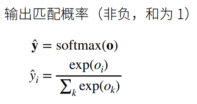
2. Define softmax operations

softmax consists of three steps: (1) exponentiation of each term (using exp); (2) Sum each row (each sample is a row in a small batch) to obtain the normalization constant of each sample; (3) Divide each row by its normalization constant to ensure that the sum of the results is 1.

def softmax(X):
    X_exp = torch.exp(X)
    partition = X_exp.sum(1, keepdim=True)
    return X_exp / partition  # The broadcast mechanism is applied here

3. Define model

The following code defines how the input is mapped to the output through the network. Note that before passing the data to our model, we use the reshape function to flatten each original image into a vector.

def net(X):
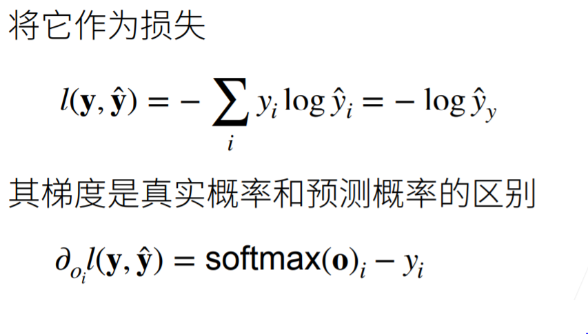
    return softmax(torch.matmul(X.reshape((-1, W.shape[0])), W) + b)

4. Define loss function

5. Classification accuracy

6. Training

7. Forecast

(7) Concise implementation of Softmax regression

2, Multilayer perceptron

(1) Multilayer perceptron

  (2) Implementation of multi-layer perceptron

1. Initialize model parameters

num_inputs, num_outputs, num_hiddens = 784, 10, 256

W1 = nn.Parameter(torch.randn(
    num_inputs, num_hiddens, requires_grad=True) * 0.01)
b1 = nn.Parameter(torch.zeros(num_hiddens, requires_grad=True))
W2 = nn.Parameter(torch.randn(
    num_hiddens, num_outputs, requires_grad=True) * 0.01)
b2 = nn.Parameter(torch.zeros(num_outputs, requires_grad=True))

params = [W1, b1, W2, b2]

2. Activation function

def relu(X):
    a = torch.zeros_like(X)
    return torch.max(X, a)

3. Model

We use reshape to convert each two-dimensional image into a length of num_ Vector of inputs.

def net(X):
    X = X.reshape((-1, num_inputs))
    H = relu(X@W1 + b1)  # Here "@" represents matrix multiplication
    return (H@W2 + b2)

4. Loss function

Directly use the built-in functions in the advanced API to calculate softmax and cross entropy loss.

loss = nn.CrossEntropyLoss()

5. Training

The training process of multilayer perceptron is exactly the same as that of softmax regression. You can call the train of d2l package directly_ CH3 function.

num_epochs, lr = 10, 0.1
updater = torch.optim.SGD(params, lr=lr)
d2l.train_ch3(net, train_iter, test_iter, loss, num_epochs, updater)

  (3) Simple implementation of multi-layer perceptron

import torch
from torch import nn
from d2l import torch as d2l

Compared with the concise implementation of softmax regression, the only difference is that we have added two full connection layers (we only added one full connection layer before). The first layer is the hidden layer, which contains 256 hidden units and uses the ReLU activation function. The second layer is the output layer.

net = nn.Sequential(nn.Flatten(),
                    nn.Linear(784, 256),
                    nn.ReLU(),
                    nn.Linear(256, 10))

def init_weights(m):
    if type(m) == nn.Linear:
        nn.init.normal_(m.weight, std=0.01)

net.apply(init_weights);

batch_size, lr, num_epochs = 256, 0.1, 10
loss = nn.CrossEntropyLoss()
trainer = torch.optim.SGD(net.parameters(), lr=lr)

train_iter, test_iter = d2l.load_data_fashion_mnist(batch_size)
d2l.train_ch3(net, train_iter, test_iter, loss, num_epochs, trainer)

(4) Model selection, under fitting and over fitting

Training error: the error calculated by the model on the training data set.

Generalization error: the error calculated by the model on the new data set.

Validation dataset: a dataset used to evaluate the quality of the model.

Test data set: a data set used only once.

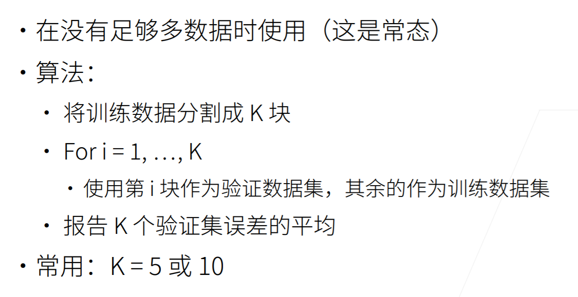
k-fold cross validation method:

  Overfitting:

Under fit:

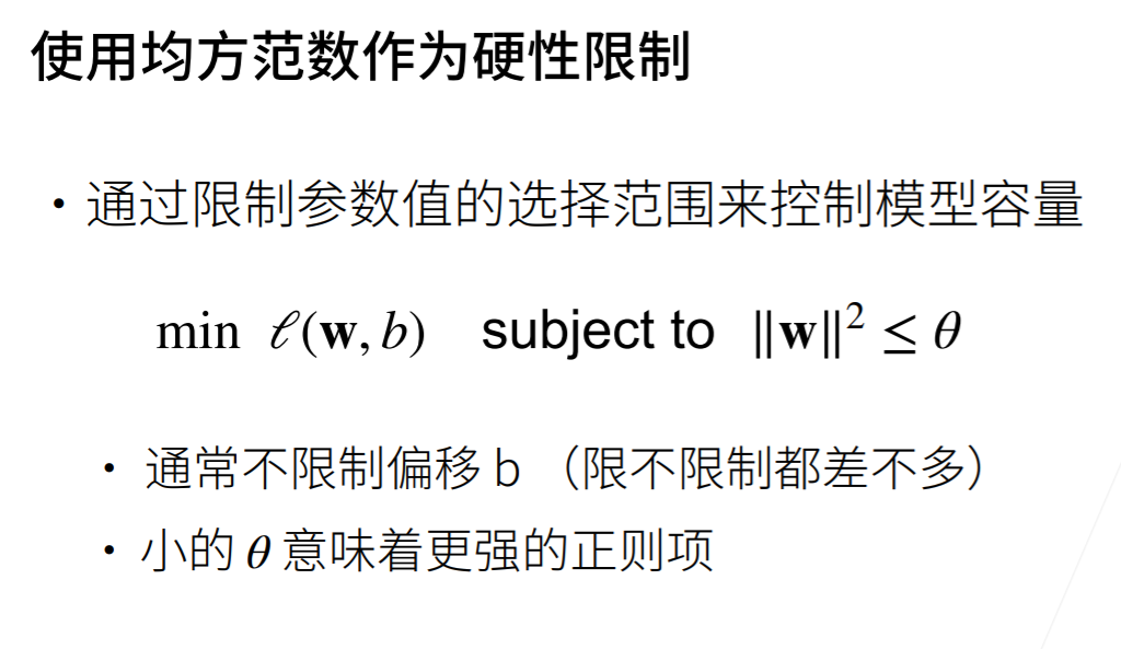
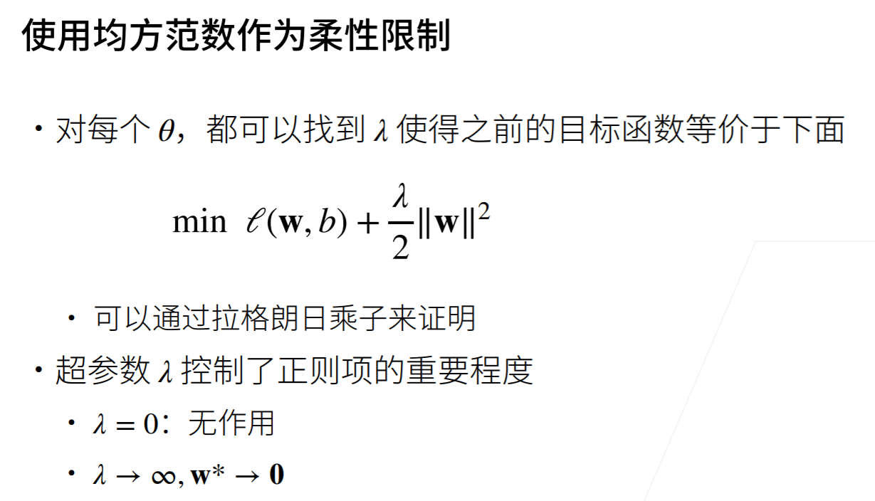
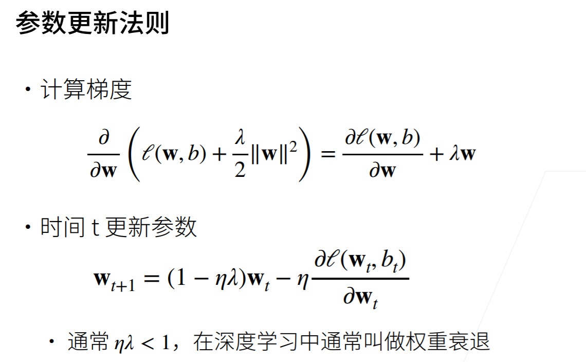
(5) Weight attenuation

 

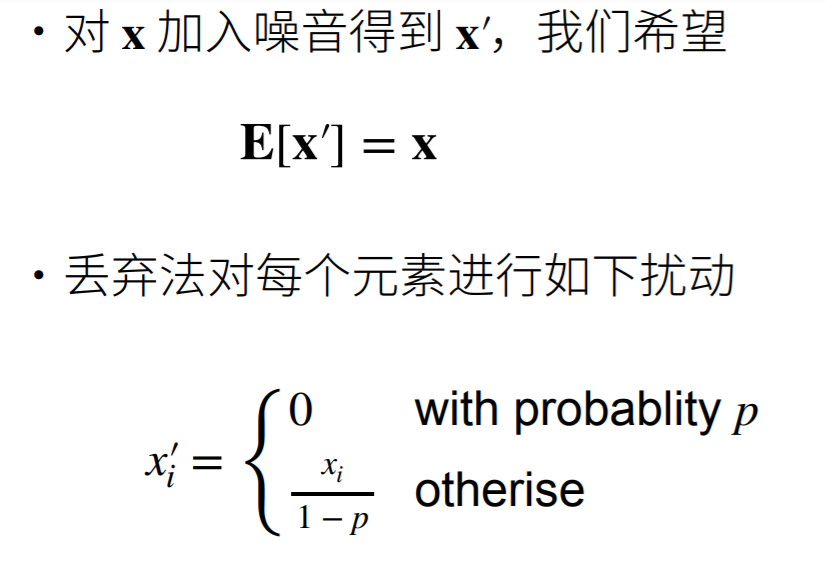
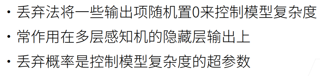
(6) Dropout