Course directory index

Chapter I course overview.
Chapter II control equipment
Chapter III control instruments
Chapter IV control software
Chapter V comprehensive case I
Section 5.2 application kit for amplitude and phase weighting.
Chapter VI comprehensive case II
Chapter VII comprehensive case III
Chapter VIII course summary

5.2.1 phased array toolkit of MATLAB

According to the analysis in the previous section, in order to finally complete the analysis of 4 × 4 phase and attenuation configuration of 16 groups of wave control chips (including NC phase shifter, NC attenuator and SPI interface). The first problem to be solved is how to obtain the required phase value matrix and attenuation value matrix.

This problem can actually be transformed into implementing two independent functions:

• The phase shift value is used to solve the function, input the working frequency f (unit: Hz), and the beam points to the pitch angle θ And azimuth φ (unit deg) and the array cell spacing dx and dy (unit mm) to obtain the phase value matrix;

• Attenuation value solution function, input window function type and amplitude lobe suppression demand to obtain attenuation value matrix.

Note that in the actual engineering application, these two functions should be embedded into the MCU and DSP inside the component through the C language algorithm. However, we use a simple but effective solution and directly call the toolkit of Matlab to solve it.

The Sensor Array Analyzer application (Phased Array System Toolbox 4.2) in Matlab version R2019b (9.7.0.1190202) is adopted. In order to better observe the phenomenon through the change of pattern, a larger 16 × The array of 16 is taken as an example for demonstration. The Uniform Rectangular Array URA (Uniform Rectangular Array) based on omnidirectional antenna Isotropic is selected. Assuming that the working frequency of the array is 15GHz, in order to meet the requirements of ± 90 ° no grid lobe, the unit spacing dx=dy=10mm. Since the scanning and weighting processes are independent of each other, we do not select the weighted Taper option, but observe the beam scanning characteristics first, The settings are shown in Figure 1.

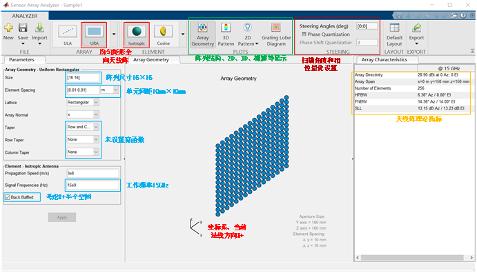
Figure 1 a 16 × 16 URA array instance

To observe the corresponding normal non scanning 3D pattern and the corresponding two-dimensional UV pattern, as shown in Figure 2.

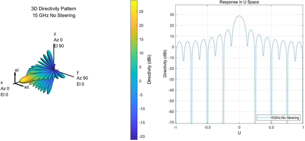
Figure 2 normal pattern (left) 3D (right) UV

By setting the beam pointing azimuth (30 °, 0 °) and pitch angle (0 °, 45 °), the change of corresponding pattern can be observed. Fig. 3 shows the scanning of azimuth, and it can be observed that the scanning is carried out in the Y-axis and X-axis planes of the coordinate system; Figure 4 shows the scanning of pitch angle. It can be observed that the scanning is carried out in the Z-axis and X-axis planes of the coordinate system.

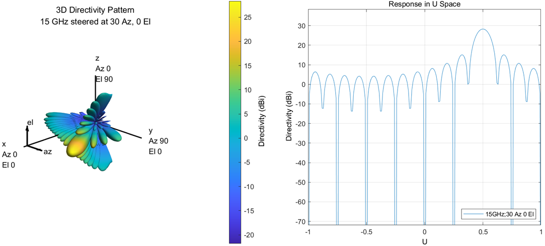
Fig. 3 azimuth scanning direction

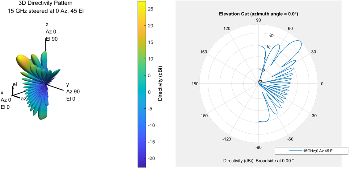
Fig. 4 scanning direction of pitch angle

After observing the beam space scanning realized by unit phase-shifting, the low amplitude lobe is realized by tower. In the pull-down menus of row tower and column tower, there are Hamming, Chebyshev, Hann, Kaiser, Taylor and Custom options (in fact, I don't know the difference between them when writing this part), Select Chebyshev and set the Sidelobe Attenuation value to 30dB (Sidelobe Attenuation). The three-dimensional and two-dimensional normal pattern are shown in Figure 5.

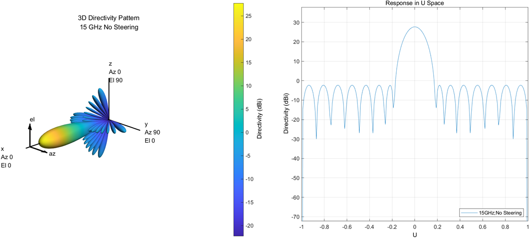
Fig. 5 normal direction after taper

In addition, pay attention to the Array Characteristics column on the right. The comparison before and after Taper is shown in Figure 6. With the improvement of SLL, that is, sidelobe suppression, the array directivity is reduced from 28.9dBi to 27.72dBi, and the beam width is widened. This is the cost of achieving low amplitude lobe.

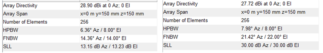
Figure 6 Comparison of array indexes before and after Taper (left) before Taper (right) after Taper

Here, we can find that the modeling, scanning and windowing of the whole array antenna can be realized by using this toolkit, but how to get the required phase and attenuation information? Next, you need to switch to the code in the background of the interface.

5.2.2 amplitude phase conversion to quantization control code

Find the Export option in the upper right corner of the interface in Figure 1. Select Generate Matlab Script from the drop-down menu to get the code. I annotated and recombined it to get the following appearance.

clear all; close all; clc;
%% Create a cell with a spacing of 10 mm Of 16×16 of URA array
Array = phased.URA('Size',[16 16],...
'Lattice','Rectangular','ArrayNormal','x');
Array.ElementSpacing = [0.01 0.01];
%% The array is composed of omnidirectional antenna elements
Elem = phased.IsotropicAntennaElement;
Elem.BackBaffled = true;
Elem.FrequencyRange = [0 15000000000];
Array.Element = Elem;
%% Calculate low amplitude lobe Taper
sll = 30;
rwind = chebwin(16, sll);
cwind = chebwin(16, sll);
taper = rwind*cwind.';
Array.Taper = taper.';
%% Calculate scan weighting
SteeringAngles = [0;0];        % Set beam scanning direction
Frequency = 15000000000;       % working frequency 
PropagationSpeed = 300000000;  % light speed
PhaseShiftBits = 0;            % Phase quantization
w = zeros(getNumElements(Array), length(Frequency));
SteerVector = phased.SteeringVector('SensorArray',Array, 'PropagationSpeed', PropagationSpeed, 'NumPhaseShifterBits', PhaseShiftBits(1));
for idx = 1:length(Frequency)
    w(:, idx) = step(SteerVector, Frequency(idx), SteeringAngles(:, idx));
end
%% Draw a three-dimensional pattern 1
Freq3D = Frequency;
format = 'polar';
Figure(1);
pattern(Array, Freq3D , 'PropagationSpeed', PropagationSpeed,...
 'Type','directivity', 'CoordinateSystem', format,'weights', w(:,1));

In order to introduce this code and help understand it, the toolkit interface is used to describe it. The toolkit interface will not be used in later programming, but this code will be mainly used.

• The w variable, which holds the phase shift information of each antenna unit in the form of imaginary number;

• And array Taper contains information about the amplitude.

The next thing to do is combine w with array Taper these two 16 × The matrix of 16 is converted into a data format that can be sent to the multi-function chip. Here, G4403 analog beamforming chip of Zhejiang Chengchang Technology Co., Ltd. is selected as an example (I have not actually used this chip, but the control methods of this kind of chip are similar). Its phase shift and attenuation truth tables are shown in Fig. 7 and Fig. 8. It can be seen that the phase shift bit is 6 bits and the step is 5.625 °. The attenuation bits are also 6 bits and the step is 0.5dB.

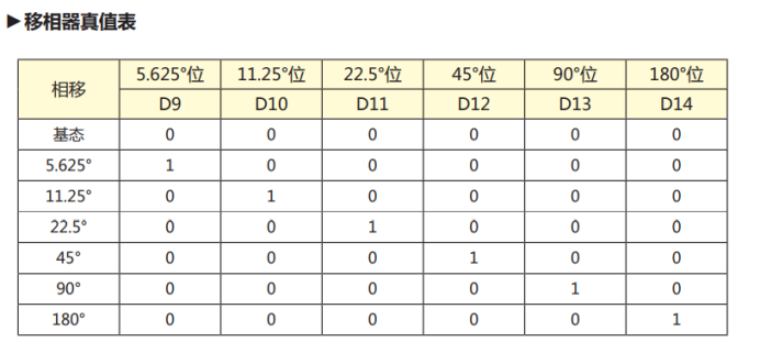
Fig. 7 truth table of g4403 phase shifter

Figure 8 truth table of g4403 attenuator

Use the following matlab code to sort out w and array The value of taper. For the phase shift value, first use the phase function of MATLAB to extract the phase of W imaginary number, then sort out the range from 0 ° to 360 ° through mod function, and finally divide it by the minimum quantization step of 5.625 °. Similarly, for the attenuation value, first convert it from the multiple value to DB, and then divide it by the minimum attenuation quantization step of 0.5dB.

%% Quantized phase and amplitude values
Phase_Shift = fix(mod(phase(w)*360/(2*pi),360)/5.625);
Att = fix(abs(10*log10(Array.Taper))/0.5);

Note that what we get here is a decimal number, which can be transformed into a binary number through the dec2bin function in matlab.

5.2.3 quantization control code verification

In order to verify the effectiveness of the conversion, recalculate the quantized phase and attenuation values through the following code, and draw the scanning 3D pattern figure 2. The correctness of this quantization conversion can be proved by comparing Figure 2 with figure 1.

%% Pattern 2 after quantization of phase and amplitude values
Array.Taper = 10.^(-Att*0.5/10);
w_ = cos(Phase_Shift*5.625*2*pi/360)+sqrt(-1)*sin(Phase_Shift*5.625*2*pi/360);
figure(2);
pattern(Array, Freq3D , 'PropagationSpeed', PropagationSpeed,...
 'Type','directivity', 'CoordinateSystem', format,'weights', w_(:,1));

If we increase the minimum step of the phase shifter to 22.5 °, what will happen if we increase the minimum step of the attenuator to 2dB? Change the above code and draw the direction diagram 3.

%% Pattern 3 after increasing phase step and attenuation step
Phase_Shift = fix(mod(phase(w)*360/(2*pi),360)/22.5);
Att = fix(abs(10*log10(taper.'))/2);
Array.Taper = 10.^(-Att*2/10);
w_ = cos(Phase_Shift*22.5*2*pi/360)+sqrt(-1)*sin(Phase_Shift*22.5*2*pi/360);
figure(3);
pattern(Array, Freq3D , 'PropagationSpeed', PropagationSpeed,...
 'Type','directivity', 'CoordinateSystem', format,'weights', w_(:,1));

The comparison of the front and rear three 3D patterns is shown in Figure 9. Adding steps will worsen the pattern, and further experiments can be carried out by changing the code.

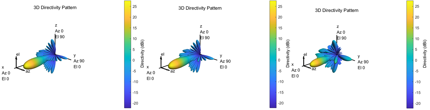
Fig. 9 (left) ideal direction diagram; (middle) 6-bit quantization pattern; (right) 4-bit quantization pattern

summary

This completes our task in this section. After a brief review, firstly, the phased array toolbox in matlab is introduced. Then, the background code is derived through modeling. The phase and attenuation values we need are obtained with the background code, and verified after quantization.