As a programmer, I have written countless confession codes to the goddess over the years. Here is a simple part to share. I hope it will help you. 520 ha ha~
Article directory:
- 1, In the simplest sentence
- 2, Python draw red hearts
- 3, Python drawing 3D red peach heart
- 4, WordCloud draws chat records belonging to two people
- 5, Using Python image processing to draw the head of the goddess
- 6, Draw filters and sketch effects belonging to the goddess
- 7, Python converts the goddess image into wonderful txt text
- 8, Using AI and Word2Vec to write poetry for the goddess
- 9, HTML confession code
1, The simplest one sentence confession
Every time I take Python data mining or big data analysis courses, I will give students a sentence to express the code, which is very simple and interesting code.
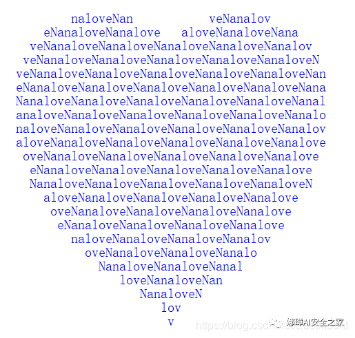
print('\n'.join([''.join([('loveNana'[(x-y)%8]if((x*0.05)**2+(y*0.1)**2-1)**3-(x*0.05)**2*(y*0.1)**3<=0 else' ')for x in range(-30,30)])for y in range(15,-15,-1)]))
The running result is shown in the figure below, and the peach heart of "lovaNana" is output.
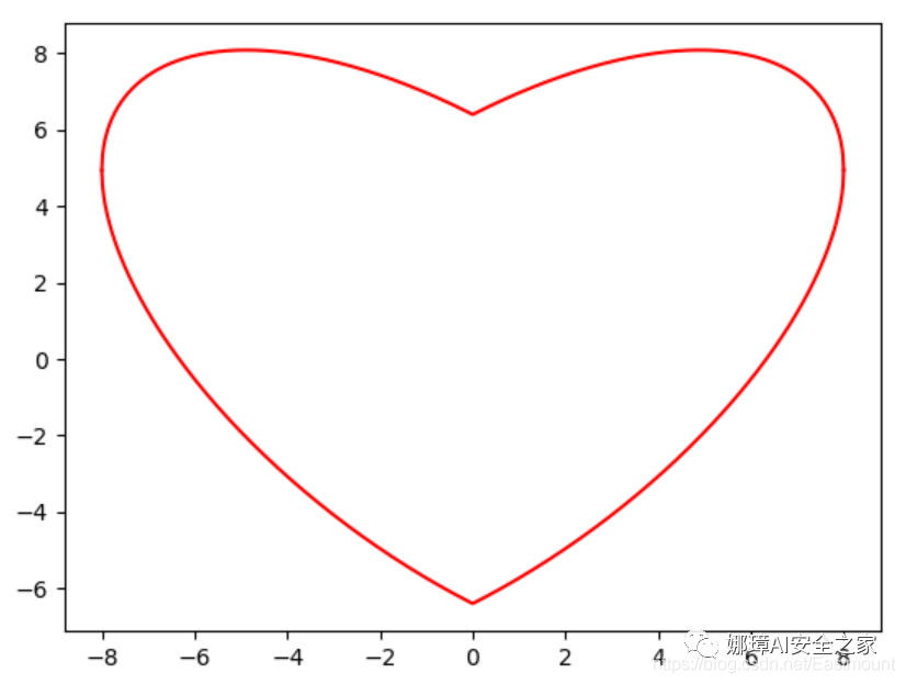
You can also call the Cartesian function to draw the peach heart, which is also an assignment assigned in my class.
import numpy as np
import matplotlib.pyplot as plt
x = np.linspace(-8 , 8, 1024)
y1 = 0.618*np.abs(x) - 0.8* np.sqrt(64-x**2)  #Left part
y2 = 0.618*np.abs(x) + 0.8* np.sqrt(64-x**2)  #Right part
plt.plot(x, y1, color = 'r')
plt.plot(x, y2, color = 'r')
plt.show()
2, Python draw red hearts
If you think the color of the above code is not festive enough, next we call the turtle library to draw the dynamic red peach heart.
from turtle import *

#Initial settings
setup(750,500)
penup()
pensize(25)
pencolor("pink")
fd(-230)
seth(90)
pendown()

#Draw peach heart
circle(-50,180)
circle(50,-180)
circle(75,-50)
circle(-190,-45)
penup()
fd(185)
seth(180)
fd(120)
seth(90)
pendown()
circle(-75,-50)
circle(190,-45)
penup()
fd(184)
seth(0)
fd(80)
seth(90)
pendown()
circle(-50,180)
circle(50,-180)
circle(75,-50)
circle(-190,-45)
penup()
fd(185)
seth(180)
fd(120)
seth(90)
pendown()
circle(-75,-50)
circle(190,-45)
penup()
fd(150)
seth(180)
fd(300)

#Draw arrow
pencolor("red")
pensize(10)
pendown()
fd(-500)
seth(90)
fd(30)
fd(-60)
seth(30)
fd(60)
seth(150)
fd(60)
done()
The operation effect is shown in the figure below:

3, Python drawing 3D red peach heart
If you think the color of the above code is not festive enough, next we call the turtle library to draw the dynamic red peach heart.
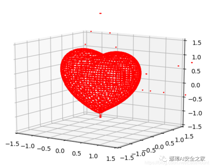
If we still feel that peach hearts are monotonous, we can draw 3D peach hearts, mainly by calling Axes3D and Matplotlib packages. The code is as follows:
#coding:utf-8
from mpl_toolkits.mplot3d import Axes3D
from matplotlib import cm
from matplotlib.ticker import LinearLocator, FormatStrFormatter
import matplotlib.pyplot as plt
import numpy as np

#Draw 3D hearts
def heart_3d(x,y,z):
    return (x**2+(9/4)*y**2+z**2-1)**3-x**2*z**3-(9/80)*y**2*z**3

#Image display
def plot_implicit(fn, bbox=(-1.5, 1.5)):
    xmin, xmax, ymin, ymax, zmin, zmax = bbox*3
    fig = plt.figure()
    ax = fig.add_subplot(111, projection='3d')
    A = np.linspace(xmin, xmax, 100)  #resolution of the contour
    B = np.linspace(xmin, xmax, 40)   #number of slices
    A1, A2 = np.meshgrid(A, A)        #grid on which the contour is plotted

    #plot contours in the XY plane
    for z in B:
        X, Y = A1, A2
        Z = fn(X, Y, z)
        cset = ax.contour(X, Y, Z+z, [z], zdir='z', colors=('r',))
        # [z] defines the only level to plot
        # for this contour for this value of z

    #plot contours in the XZ plane
    for y in B:
        X, Z = A1, A2
        Y = fn(X, y, Z)
        cset = ax.contour(X, Y+y, Z, [y], zdir='y', colors=('red',))

    #plot contours in the YZ plane
    for x in B:
        Y, Z = A1, A2
        X = fn(x, Y, Z)
        cset = ax.contour(X+x, Y, Z, [x], zdir='x',colors=('red',))

    #axis
    ax.set_zlim3d(zmin, zmax)
    ax.set_xlim3d(xmin, xmax)
    ax.set_ylim3d(ymin, ymax)

    #Display image
    plt.show()

#Main function
if __name__ == '__main__':
    plot_implicit(heart_3d)
The output results are shown in the figure below:
4, WordCloud draws two people's chat records
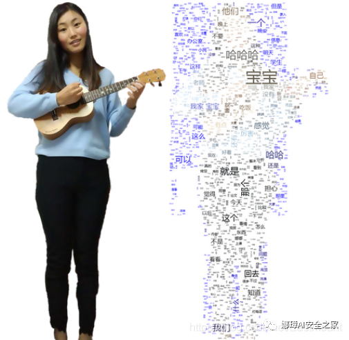
"Word cloud" is to give visual prominence to the frequently occurring keywords in the network text, so that web browsers can appreciate the theme of the text as long as they scan the text, mainly using text mining and visualization technology.
The author exports the wechat chat records of the two people, and uses the following code to draw the word cloud map belonging to the two people, of which "baby", "we" and "ha ha" are the most. If you add stop word filtering, you can see your story~
# -*- coding: utf-8 -*-
from os import path
from scipy.misc import imread
import jieba
import sys
import matplotlib.pyplot as plt
from wordcloud import WordCloud, STOPWORDS, ImageColorGenerator

# Open ontology TXT file
text = open('test.txt').read()

# Stuttering participle cut_all=True set to full mode
wordlist = jieba.cut(text)     #cut_all = True

# Chinese word segmentation using space connection
wl_space_split = " ".join(wordlist)
print(wl_space_split)

# Read mask/color pictures
d = path.dirname(__file__)
nana_coloring = imread(path.join(d, "mb.png"))

# Generate word cloud for text after word segmentation
my_wordcloud = WordCloud( background_color = 'white',
                            mask = nana_coloring,
                            max_words = 2000,
                            stopwords = STOPWORDS,
                            max_font_size = 50,
                            random_state = 30,
                            )

# generate word cloud
my_wordcloud.generate(wl_space_split)

# create coloring from image
image_colors = ImageColorGenerator(nana_coloring)

# recolor wordcloud and show
my_wordcloud.recolor(color_func=image_colors)

plt.imshow(my_wordcloud)    # Show word cloud
plt.axis("off")             # Whether to display x-axis and y-axis Subscripts
plt.show()

# save img
my_wordcloud.to_file(path.join(d, "cloudimg.png"))

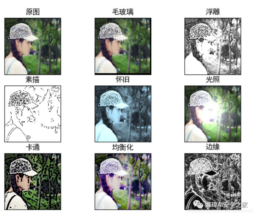
5, Image processing to draw the head of the goddess
The author shared image processing before. Similarly, we can make various image processing with Python and define a PS tool for the goddess. Relevant codes are shared here:
#encoding:utf-8
#By:Eastmount CSDN 2021-02-06
import cv2
import numpy as np
import matplotlib.pyplot as plt
import matplotlib
import math

#Read picture
img = cv2.imread('na.png')
src = cv2.cvtColor(img, cv2.COLOR_BGR2RGB)

#New target image
dst1 = np.zeros_like(img)

#Get image rows and columns
rows, cols = img.shape[:2]

#--------------------------------Ground glass effect-----------------------------------
#The color of the random pixel in the neighborhood of the pixel replaces the color of the current pixel
offsets = 5
random_num = 0
for y in range(rows - offsets):
    for x in range(cols - offsets):
        random_num = np.random.randint(0,offsets)
        dst1[y,x] = src[y + random_num,x + random_num]

#--------------------------------Paint effects-------------------------------------
#Image gray processing
gray = cv2.cvtColor(img,cv2.COLOR_BGR2GRAY)

#Custom convolution kernel
kernel = np.array([[-1,-1,-1],[-1,10,-1],[-1,-1,-1]])

#Image relief effect
dst2 = cv2.filter2D(gray, -1, kernel)

#--------------------------------Sketch effects-------------------------------------
#Gaussian filter noise reduction
gaussian = cv2.GaussianBlur(gray, (5,5), 0)

#edge detection
canny = cv2.Canny(gaussian, 50, 150)

#Threshold processing
ret, dst3 = cv2.threshold(canny, 100, 255, cv2.THRESH_BINARY_INV)

#--------------------------------Nostalgic effects-------------------------------------
#New target image
dst4 = np.zeros((rows, cols, 3), dtype="uint8")

#Image nostalgic effects
for i in range(rows):
    for j in range(cols):
        B = 0.272*img[i,j][2] + 0.534*img[i,j][1] + 0.131*img[i,j][0]
        G = 0.349*img[i,j][2] + 0.686*img[i,j][1] + 0.168*img[i,j][0]
        R = 0.393*img[i,j][2] + 0.769*img[i,j][1] + 0.189*img[i,j][0]
        if B>255:
            B = 255
        if G>255:
            G = 255
        if R>255:
            R = 255
        dst4[i,j] = np.uint8((B, G, R))

#--------------------------------Lighting effects-------------------------------------
#Set center point
centerX = rows / 2
centerY = cols / 2
print(centerX, centerY)
radius = min(centerX, centerY)
print(radius)

#Set light intensity
strength = 200

#New target image
dst5 = np.zeros((rows, cols, 3), dtype="uint8")

#Image lighting effects
for i in range(rows):
    for j in range(cols):
        #Calculates the distance from the current point to the lighting Center (the distance between two points in a planar coordinate system)
        distance = math.pow((centerY-j), 2) + math.pow((centerX-i), 2)
        #Get original image
        B =  src[i,j][0]
        G =  src[i,j][1]
        R = src[i,j][2]
        if (distance < radius * radius):
            #The enhanced illumination value is calculated according to the distance
            result = (int)(strength*( 1.0 - math.sqrt(distance) / radius ))
            B = src[i,j][0] + result
            G = src[i,j][1] + result
            R = src[i,j][2] + result
            #Judge the boundary to prevent crossing the boundary
            B = min(255, max(0, B))
            G = min(255, max(0, G))
            R = min(255, max(0, R))
            dst5[i,j] = np.uint8((B, G, R))
        else:
            dst5[i,j] = np.uint8((B, G, R))

#--------------------------------Nostalgic effects-------------------------------------
#New target image
dst6 = np.zeros((rows, cols, 3), dtype="uint8")

#Image fleeting effect
for i in range(rows):
    for j in range(cols):
        #The square of the value of channel B is multiplied by parameter 12
        B = math.sqrt(src[i,j][0]) * 12
        G =  src[i,j][1]
        R =  src[i,j][2]
        if B>255:
            B = 255
        dst6[i,j] = np.uint8((B, G, R))

#--------------------------------Cartoon effects-------------------------------------
#Defines the number of bilateral filters
num_bilateral = 7

#Reduce sampling with Gaussian pyramid
img_color = src

#Bilateral filtering processing
for i in range(num_bilateral):
    img_color = cv2.bilateralFilter(img_color, d=9, sigmaColor=9, sigmaSpace=7)

#Gray image conversion
img_gray = cv2.cvtColor(src, cv2.COLOR_RGB2GRAY)

#Median filter processing
img_blur = cv2.medianBlur(img_gray, 7)

#Edge detection and adaptive thresholding
img_edge = cv2.adaptiveThreshold(img_blur, 255,
                                 cv2.ADAPTIVE_THRESH_MEAN_C,
                                 cv2.THRESH_BINARY,
                                 blockSize=9,
                                 C=2)

#Convert back to color image
img_edge = cv2.cvtColor(img_edge, cv2.COLOR_GRAY2RGB)

#And operation
dst6 = cv2.bitwise_and(img_color, img_edge)

#--------------------------------Equalization effect-------------------------------------
#New target image
dst7 = np.zeros((rows, cols, 3), dtype="uint8")

#Extract three color channels
(b, g, r) = cv2.split(src)

#Color image equalization
bH = cv2.equalizeHist(b)
gH = cv2.equalizeHist(g)
rH = cv2.equalizeHist(r)

#Merge channel
dst7 = cv2.merge((bH, gH, rH))

#--------------------------------Edge effect-------------------------------------
#Gaussian filter noise reduction
gaussian = cv2.GaussianBlur(gray, (3,3), 0)

#edge detection
#dst8 = cv2.Canny(gaussian, 50, 150)

# Scharr operator
x = cv2.Scharr(gaussian, cv2.CV_32F, 1, 0) #X direction
y = cv2.Scharr(gaussian, cv2.CV_32F, 0, 1) #Y direction
absX = cv2.convertScaleAbs(x)
absY = cv2.convertScaleAbs(y)
dst8 = cv2.addWeighted(absX, 0.5, absY, 0.5, 0)

#-----------------------------------------------------------------------------
#Used to display Chinese labels normally
plt.rcParams['font.sans-serif']=['SimHei']

#Cycle through graphics
titles = [ 'Original drawing', 'Ground glass', 'relief', 'Sketch', 'Nostalgia', 'illumination', 'Cartoon', 'Equalization', 'edge']
images = [src, dst1, dst2, dst3, dst4, dst5, dst6, dst7, dst8]
for i in range(9):
   plt.subplot(3, 3, i+1), plt.imshow(images[i],'gray')
   plt.title(titles[i])
   plt.xticks([]),plt.yticks([])
plt.show()
The output results are shown in the figure below, including ground glass, paint, sketch, nostalgia, lighting, cartoon, equalization and edge effects.
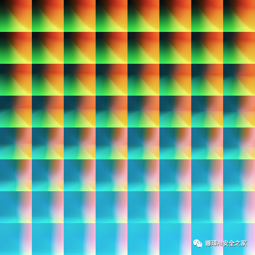
6, Draw filters and sketch effects belonging to the goddess
Sketch and filter are two great effects, which can also be implemented in Python code.
#coding:utf-8
import cv2
import numpy as np

def dodgeNaive(image, mask):
    # determine the shape of the input image
    width, height = image.shape[:2]

    # prepare output argument with same size as image
    blend = np.zeros((width, height), np.uint8)

    for col in range(width):
        for row in range(height):
            # do for every pixel
            if mask[col, row] == 255:
                # avoid division by zero
                blend[col, row] = 255
            else:
                # shift image pixel value by 8 bits
                # divide by the inverse of the mask
                tmp = (image[col, row] << 8) / (255 - mask)
                # print('tmp={}'.format(tmp.shape))
                # make sure resulting value stays within bounds
                if tmp.any() > 255:
                    tmp = 255
                    blend[col, row] = tmp
    return blend

def dodgeV2(image, mask):
    return cv2.divide(image, 255 - mask, scale=256)

def burnV2(image, mask):
    return 255 - cv2.divide(255 - image, 255 - mask, scale=256)

def rgb_to_sketch(src_image_name, dst_image_name):
    img_rgb = cv2.imread(src_image_name)
    img_gray = cv2.cvtColor(img_rgb, cv2.COLOR_BGR2GRAY)
    # Direct conversion operation when reading pictures
    # img_gray = cv2.imread('example.jpg', cv2.IMREAD_GRAYSCALE)

    img_gray_inv = 255 - img_gray
    img_blur = cv2.GaussianBlur(img_gray_inv, ksize=(21, 21),
                                sigmaX=0, sigmaY=0)
    img_blend = dodgeV2(img_gray, img_blur)

    cv2.imshow('original', img_rgb)
    cv2.imshow('gray', img_gray)
    cv2.imshow('gray_inv', img_gray_inv)
    cv2.imshow('gray_blur', img_blur)
    cv2.imshow("pencil sketch", img_blend)
    cv2.waitKey(0)
    cv2.destroyAllWindows()
    cv2.imwrite(dst_image_name, img_blend)

if __name__ == '__main__':
    src_image_name = 'nv.png'
    dst_image_name = 'sketch_example.jpg'
    rgb_to_sketch(src_image_name, dst_image_name)
The running results are shown in the figure below. We can draw notes according to the sketch. I have also painted several copies for the goddess over the years, ha ha.

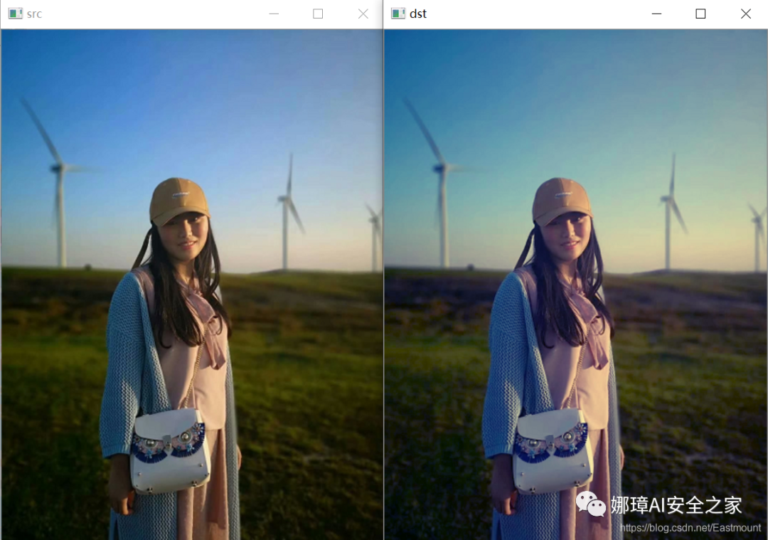
Similarly, through the filter template below, we can make the color of the picture more saturated.
#coding:utf-8
#By:Eastmount CSDN 2020-12-22
import cv2
import math
import numpy as np

#Read original image
img = cv2.imread('nv.png')

#Get image rows and columns
rows, cols = img.shape[:2]

#New target image
dst = np.zeros((rows, cols, 3), dtype="uint8")

#Image fleeting effect
for i in range(rows):
    for j in range(cols):
        #The square of the value of channel B is multiplied by parameter 12
        B = math.sqrt(img[i,j][0]) * 12
        G =  img[i,j][1]
        R =  img[i,j][2]
        if B>255:
            B = 255
        dst[i,j] = np.uint8((B, G, R))

#Display image
cv2.imshow('src', img)
cv2.imshow('dst', dst)

cv2.waitKey()
cv2.destroyAllWindows()
The output results are shown in the figure below:
7, The goddess image is converted into wonderful txt text
The code is as follows:
# -*- coding: utf-8 -*-
"""
Created on Sun Oct 23 12:45:47 2016
@author: yxz15
"""

from PIL import Image
import os

serarr=['@','#','$','%','&','?','*','o','/','{','[','(','|','!','^','~','-','_',':',';',',','.','`',' ']
count=len(serarr)

def toText(image_file):
   image_file=image_file.convert("L")#Turn gray
   asd =''#Save string
   for h in range(0,  image_file.size[1]):#h
      for w in range(0, image_file.size[0]):#w
         gray =image_file.getpixel((w,h))
         asd=asd+serarr[int(gray/(255/(count-1)))]
      asd=asd+'\r\n'
   return asd

def toText2(image_file):
   asd =''#Save string
   for h in range(0,  image_file.size[1]):#h
      for w in range(0, image_file.size[0]):#w
         r,g,b =image_file.getpixel((w,h))
         gray =int(r* 0.299+g* 0.587+b* 0.114)
         asd=asd+serarr[int(gray/(255/(count-1)))]
      asd=asd+'\r\n'
   return asd


image_file = Image.open("nana.jpg") # Open picture
image_file=image_file.resize((int(image_file.size[0]*0.9), int(image_file.size[1]*0.5)))#size pictures

print('Info:',image_file.size[0],' ',image_file.size[1],' ',count)

try:
   os.remove('./tmp.txt')
except  WindowsError:
    pass

tmp=open('tmp.txt','a')


tmp.write(toText2(image_file))

tmp.close()
The output result is shown in the figure below. Put my silly photo.

8, AI and Word2Vec wrote poems for the goddess
The basic process is as follows:
- Firstly, there is a "ancient poetry. txt" data set, which contains 43101 poems, which is used for training
- Then, read the ancient poetry data through ls_of_ls_of_c = [list(line.strip()) for line in f] code splits ancient poetry into a single word, and the words in each poem have context
- Then, call Word2Vec to train, convert to word vector and save the model.
- Finally, input the title for completion, search the semantics according to the four words of the title, calculate the similarity of each word, and finally form the corresponding poem. The core code is:
model.predict_output_word(poem[-self.window:],
max(self.topn, len(poem) + 1))
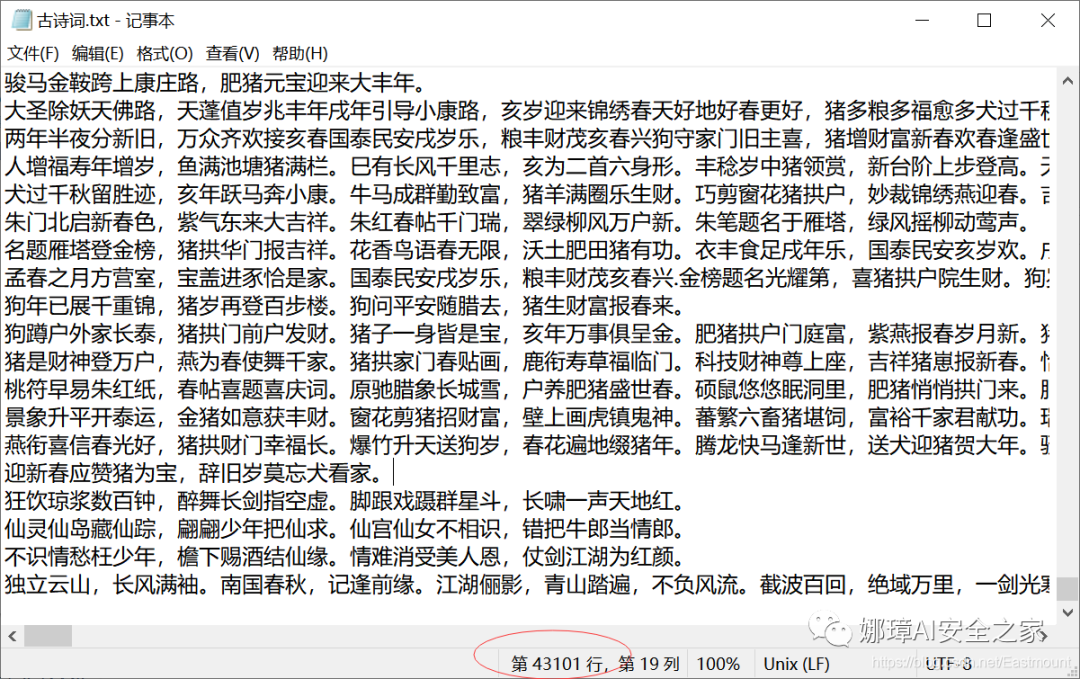
The operation results are shown in the figure below:
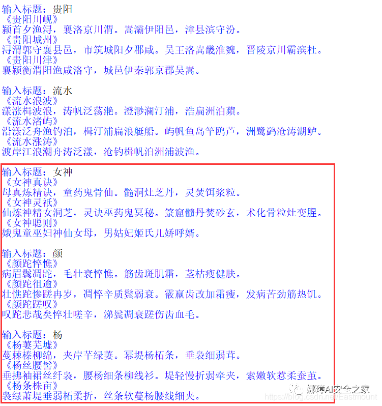
For example, input the goddess's surname "Yan", and the output five character quatrains and seven strict quatrains are as follows. Note that "withered eyebrows and temples" can not be found in our "ancient poetry. txt", but because "withered" and "Na" have similar semantics. At the same time, some words may not exist, so we need to enrich the text library.
Enter Title: Yan
<"Gaunt and haggard"
The sick eyebrows and temples wither, and the hair is strong, withered and haggard. Tendons and teeth spot cream, thin stems and healthy skin.
<"Yan Wanyu"
Strong and gaunt, miserable and old, withered and pungent, weak temples. Graupel teeth are changed to frost and thin, and the disease is bitter, strong, hot and hungry.
<"Yan wasted sigh"
Sigh, it's sad. It's haggard, strong and pungent. The tears on the temples wither and hurt the teeth and blood hair.
The complete code is as follows:
# -*- coding: utf-8 -*-
"""
Created on Mon Dec 23 17:48:50 2019
@author: xiuzhang Eastmount CSDN

Blog original address: https://blog.csdn.net/Yellow_python/article/details/86726619
 I recommend you to study Yellow_python Great God's article
"""
from gensim.models import Word2Vec  # Word vector
from random import choice
from os.path import exists

class CONF:
    path = 'Ancient poetry.txt'
    window = 16           # Sliding window size
    min_count = 60        # Filter low frequency words
    size = 125            # Word vector dimension
    topn = 14             # Openness of generative Poetry
    model_path = 'word2vec'

# Define model
class Model:
    def __init__(self, window, topn, model):
        self.window = window
        self.topn = topn
        self.model = model  # Word vector model
        self.chr_dict = model.wv.index2word  # Dictionaries

    """Model initialization"""
    @classmethod
    def initialize(cls, config):
        if exists(config.model_path):
            # Model reading
            model = Word2Vec.load(config.model_path)
        else:
            # Corpus reading
            with open(config.path, encoding='utf-8') as f:
                ls_of_ls_of_c = [list(line.strip()) for line in f]
            # Model training and preservation
            model = Word2Vec(sentences=ls_of_ls_of_c, size=config.size, window=config.window, min_count=config.min_count)
            model.save(config.model_path)
        return cls(config.window, config.topn, model)

    """Generation of ancient poetry"""
    def poem_generator(self, title, form):
        filter = lambda lst: [t[0] for t in lst if t[0] not in [',', '. ']]
        # Title completion
        if len(title) < 4:
            if not title:
                title += choice(self.chr_dict)
            for _ in range(4 - len(title)):
                similar_chr = self.model.similar_by_word(title[-1], self.topn // 2)
                similar_chr = filter(similar_chr)
                char = choice([c for c in similar_chr if c not in title])
                title += char

        # Text generation
        poem = list(title)
        for i in range(form[0]):
            for _ in range(form[1]):
                predict_chr = self.model.predict_output_word(poem[-self.window:], max(self.topn, len(poem) + 1))
                predict_chr = filter(predict_chr)
                char = choice([c for c in predict_chr if c not in poem[len(title):]])
                poem.append(char)
            poem.append(',' if i % 2 == 0 else '. ')
        length = form[0] * (form[1] + 1)
        return '<%s>' % ''.join(poem[:-length]) + '\n' + ''.join(poem[-length:])


def main(config=CONF):
    form = {'Five character quatrains': (4, 5), 'four-line poem with seven characters per line': (4, 7), 'Couplet': (2, 9)}
    m = Model.initialize(config)
    while True:
        title = input('Enter Title:').strip()
        try:
            poem = m.poem_generator(title, form['Five character quatrains'])
            print('%s' % poem)  # red
            poem = m.poem_generator(title, form['four-line poem with seven characters per line'])
            print('%s' % poem)  # yellow
            poem = m.poem_generator(title, form['Couplet'])
            print('%s' % poem)  # purple
            print()
        except:
            pass

if __name__ == '__main__':
    main()
PS: yellow is referenced in this section_ Python great God's blog recommends artificial intelligence children's shoes to learn his articles. It's really good.
9, HTML confession code
In addition to Python, various programming languages can make exquisite confession code. The following code of HTML5 is supplemented for everyone to learn. Of course, there are many open sources on the Internet. All the code in this article can be downloaded from the following link.
- https://github.com/eastmountyxz/Love-code