1 Overview

1.1 what are the sub warehouse and sub table

Xiao Ming is a developer of a start-up e-commerce platform. He is responsible for the function development of the seller module,
The related businesses of shops and commodities are involved, and the design is as follows
Database:

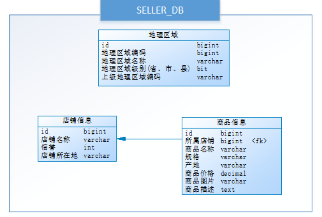
Store information and geographical area information related to goods can be obtained through the following SQL:

SELECT p.*,r.[Geographical area name],s.[Shop name],s.[reputation]
FROM [Commodity information] p
LEFT JOIN [Geographical area] r ON p.[Place of Origin] = r.[Geographical area coding]
LEFT JOIN [Store information] s ON p.id = s.[Store]
WHERE p.id = ?

Form a list similar to the following:

With the rapid development of the company's business, the amount of data in the database increases sharply, and the access performance slows down. Optimization is imminent. Analyze where the problem is? Relational database itself is easy to become a system bottleneck, and the storage capacity, connection number and processing capacity of a single machine are limited. When the data volume of a single table reaches 1000W or 100G, due to the large number of query dimensions, the performance still degrades seriously even when adding slave databases and optimizing indexes.

• Option 1:
  Improve the data processing capacity by improving the hardware capacity of the server, such as increasing storage capacity and CPU. This scheme costs a lot, and if the bottleneck is MySQL itself, it is also helpful to improve the hardware.

• Option 2:
  Disperse the data in different databases to reduce the amount of data in a single database, so as to alleviate the performance problem of a single database, so as to improve the performance of the database. As shown in the figure below, the e-commerce database is divided into several independent databases, and the large table is also divided into several small tables, This method of database splitting is used to solve the performance problem of database.

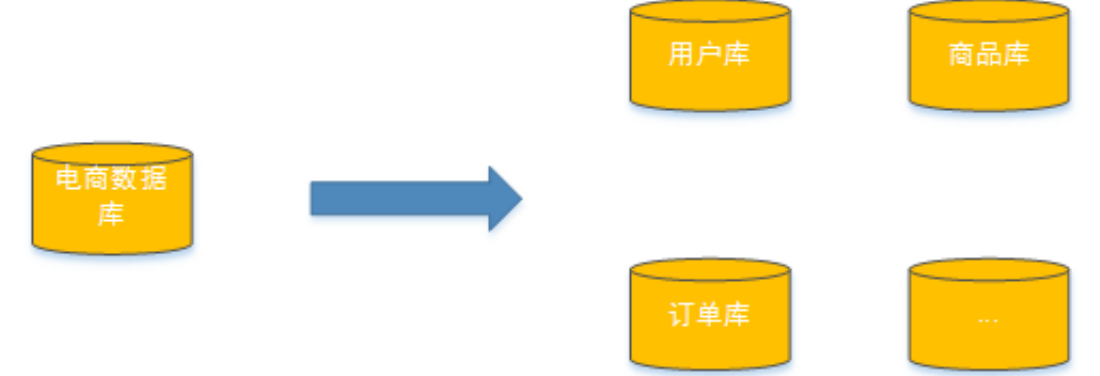
Database and table splitting is to solve the problem of database performance degradation due to excessive amount of data. The original independent database is divided into several databases, and the large data table is divided into several data tables, so as to reduce the amount of data in a single database and single data table, so as to improve the performance of the database.

1.2 method of warehouse and table division

The sub warehouse and sub table includes two parts: sub warehouse and sub table. In production, it usually includes four methods: vertical sub warehouse, horizontal sub warehouse, vertical sub table and horizontal sub table.

1.2.1 vertical sub table

The following is a case of commodity query to explain the vertical sub table:
The details of goods are usually not displayed in the following list:

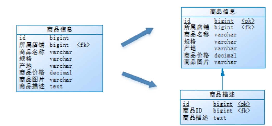
When browsing the product list, users will view the detailed description of a product only when they are interested in it. Therefore, the access frequency of the commodity description field in the commodity information is low, the storage space of this field is large, and the IO time of accessing a single data is long; The data access frequency of other fields such as commodity name, commodity picture and commodity price in commodity information is high.

Because the characteristics of the two data are different, he considered splitting the commodity information table as follows:

The product description information with low access frequency is stored in a separate table, and the basic information of products with high access frequency is placed in a separate table.

The commodity list can adopt the following sql:

SELECT p.*,r.[Geographical area name],s.[Shop name],s.[reputation]
FROM [Commodity information] p
LEFT JOIN [Geographical area] r ON p.[Place of Origin] = r.[Geographical area coding]
LEFT JOIN [Store information] s ON p.id = s.[Store]
WHERE...ORDER BY...LIMIT...

When the product description needs to be obtained, it can be obtained through the following sql:

SELECT *
FROM [Product description]
WHERE [commodity ID] = ?

This step of optimization carried out by Xiao Ming is called vertical sub table.
Vertical table division definition: divide a table into multiple tables according to fields, and each table stores some of the fields.

The improvement brought by vertical sub table is:

1. In order to avoid IO contention and reduce the probability of locking the table, users who view details and commodity information browsing do not affect each other
2. Give full play to the operation efficiency of popular data, and the high efficiency of commodity information operation will not be dragged down by the low efficiency of commodity description.

Generally speaking, the access frequency of each data item in a business entity is different. Some data items may be blobs or TEXT that occupy a large storage space. For example, the product description in the above example. Therefore, when the amount of data in the table is large, the table can be
Cut by field, and place the popular fields and unpopular fields in different libraries separately. These libraries can be placed on different storage devices to avoid IO competition. The performance improvement brought by vertical segmentation mainly focuses on the operation efficiency of hot data, and the disk contention is reduced.

We usually split vertically according to the following principles:

1. Put the uncommon fields in a separate table;
2. Split text, blob and other large fields and put them in the attached table;
3. The columns of frequent combined queries are placed in one table;

1.2.2 vertical sub warehouse

The performance of vertical table splitting has been improved to a certain extent, but it has not met the requirements, and the disk space is not fast enough. Because the data is always limited to one server, the vertical table splitting in the library only solves the problem of excessive data of a single table, but does not distribute the tables to different servers. Therefore, each table still competes for the CPU, memory and Network IO, disk.

After thinking, he put the original seller_ DB (seller Library), divided into product_ DB and store_ DB (store library) and distribute the two libraries to different servers, as shown in the following figure:

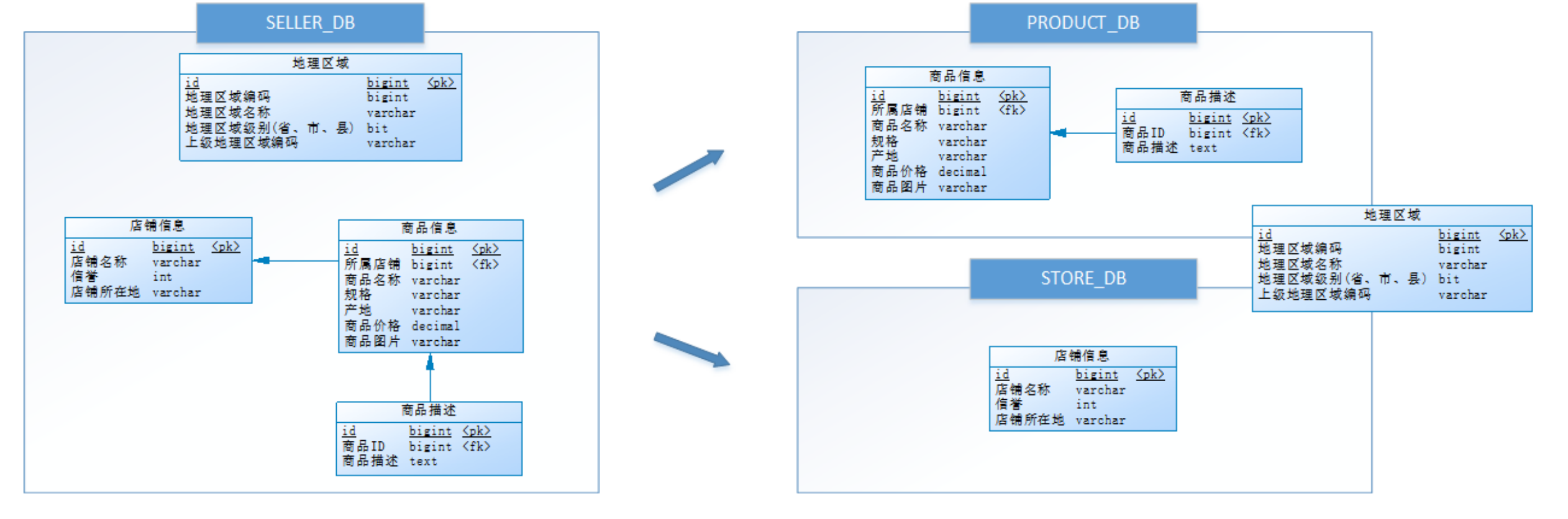
Due to the high coupling between commodity information and commodity description business, it is stored in product together_ DB (commodity warehouse); The store information is relatively independent, so it is stored separately in the store_ DB (store library).

This step of optimization carried out by Xiao Ming is called vertical sub database.

Vertical sub database refers to classifying tables according to business and distributing them to different databases. Each database can be placed on different servers. Its core concept is special database.

The improvements it brings are:

1. Solve the coupling at the business level and make the business clear
2. It can manage, maintain, monitor and expand the data of different businesses at different levels
3. In the high concurrency scenario, the vertical sub database can increase the number of IO and database connections to a certain extent and reduce the bottleneck of single machine hardware resources

By classifying the tables according to business and then distributing them in different databases, the vertical sub database can deploy these databases on different servers, so as to achieve the effect of sharing the pressure of multiple servers, but it still does not solve the problem of too much data in a single table.

1.2.3 horizontal sub warehouse

With the increase of the business volume of product, the performance of the database will be improved to a certain extent_ The data stored in dB (commodity warehouse) single warehouse has exceeded the estimate. It is roughly estimated that there are 8w stores at present, with an average of 150 per store
For commodities of different specifications, if the growth is included, the quantity of commodities must be estimated at 1500w + and product_ DB (commodity Library) is a resource that is accessed frequently and cannot be supported by a single server. What should I do now

Optimization?
Again? However, from the perspective of business, the current situation has been unable to divide the database vertically again. Try to divide the stores horizontally, and put the commodity information with odd store ID and even store ID into two libraries respectively.

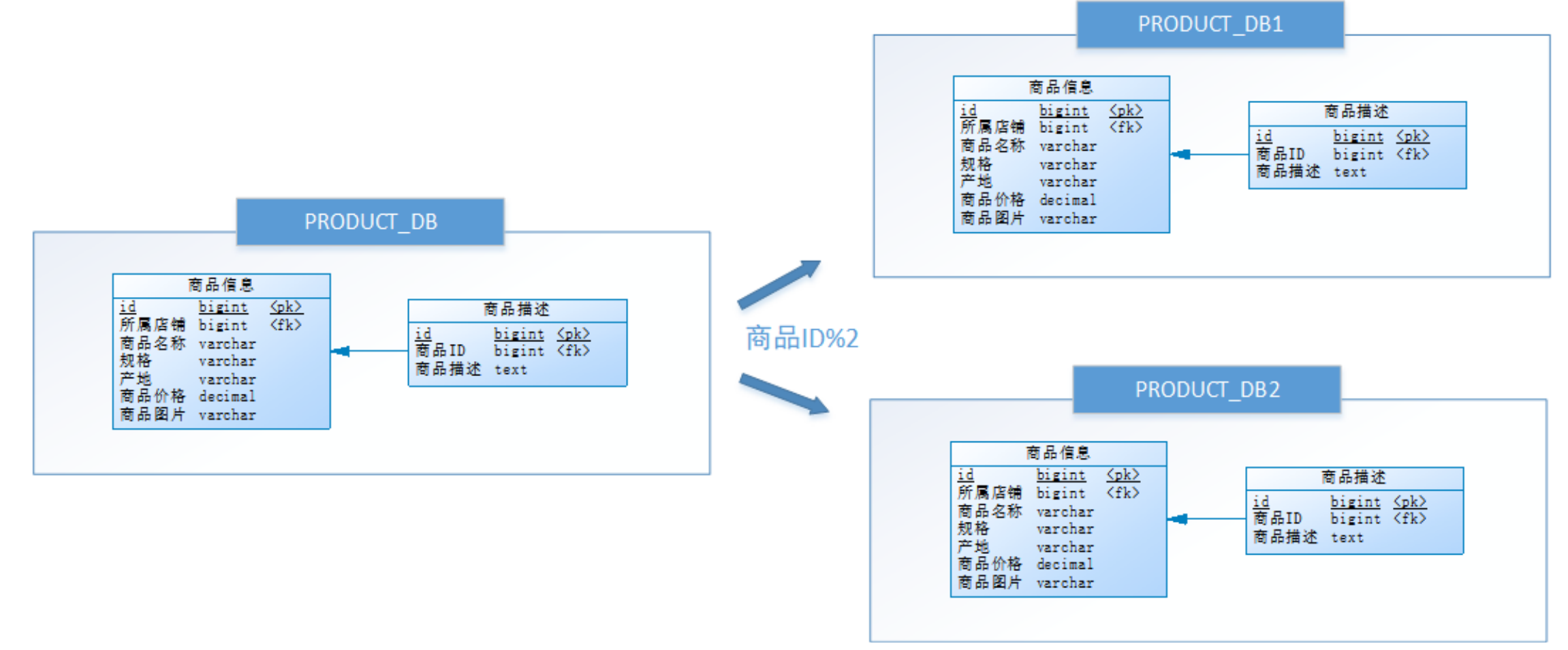
In other words, to operate a piece of data, first analyze the store ID to which the data belongs. If the store ID is an even number, map this operation to RRODUCT_DB1 (commodity warehouse 1); If the store ID is singular, map the operation to RRODUCT_DB2 (commodity library 2). The expression to access the database name for this operation is RRODUCT_DB [store ID%2 + 1].

This step of optimization carried out by Xiao Ming is called horizontal sub database.

Horizontal sub database: it is to split the data of the same table into different databases according to certain rules, and each database can be placed on different servers.

The improvement brought by horizontal sub warehouse is:

1. It solves the performance bottleneck of single database, big data and high concurrency.
2. The stability and availability of the system are improved.

When an application is difficult to perform fine-grained vertical segmentation, or the number of rows of data after segmentation is huge, and there is a bottleneck in the reading, writing and storage performance of a single database, it is necessary to perform horizontal segmentation. After the optimization of horizontal segmentation, the bottleneck of single inventory reserves and performance can often be solved. However, because the same table is assigned to different databases, additional routing of data operation is required, which greatly improves the complexity of the system.

1.2.4 horizontal sub table

According to the idea of horizontal sub library, product_ DB_ The tables in X (commodity Library) can also be split horizontally. The purpose is to solve the problem of large amount of data in a single table, as shown in the following figure:

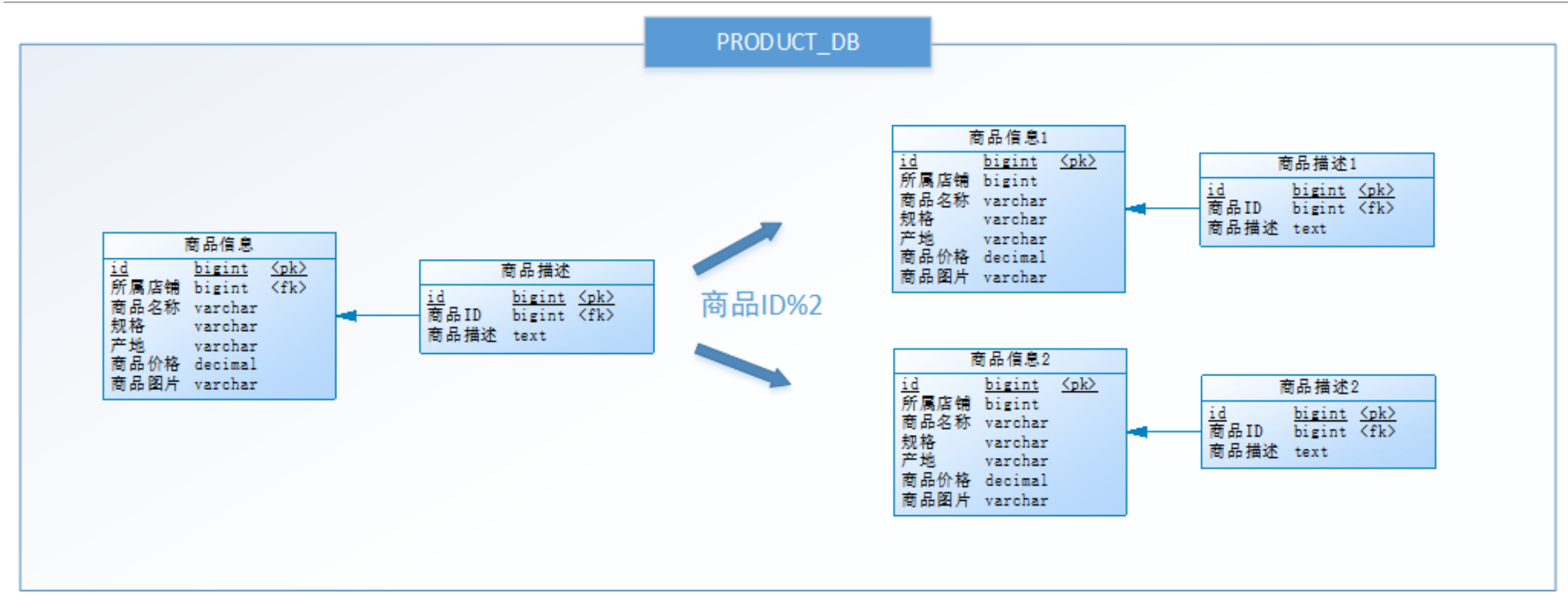
It is similar to the idea of horizontal sub database, but the goal of this operation is table. Commodity information and commodity description are divided into two sets of tables. If the commodity ID is an even number, map this operation to the commodity information 1 table; If the item ID is singular, map the operation to the item information 2 table. The expression to access the table name for this operation is product information [product ID%2 + 1].

This step of optimization carried out by Xiao Ming is called horizontal sub table.

Horizontal split table is to split the data of the same table into multiple tables according to certain rules in the same database.

The improvement level is:

1. Optimize the performance problems caused by the large amount of data in a single table
2. Avoid IO contention and reduce the probability of locking the table

The horizontal table division in the library solves the problem that the data volume of a single table is too large. The separated small table contains only part of the data, which makes the data volume of a single table smaller and improves the retrieval performance.

1.2.5 summary

This chapter introduces various methods of sub database and sub table, including vertical sub table, vertical sub database, horizontal sub database and horizontal sub table:

1. Vertical table splitting: the fields of a wide table can be divided into multiple tables according to the access frequency and whether they are large fields. This can not only make the business clear, but also improve some performance. After splitting, try to avoid associated queries from a business perspective, otherwise the performance will be poor
   The gains will outweigh the losses.
2. Vertical sub database: multiple tables can be classified according to the tightness of business coupling and stored in different libraries. These libraries can be distributed in different servers, so that the access pressure is loaded by multiple servers, greatly improving the performance, and improving the business clarity of the overall architecture. Different business libraries can customize optimization schemes according to their own conditions. But it needs to solve all the complex problems caused by cross library.
3. Horizontal sub database: the data of a table (by data row) can be divided into multiple different databases. Each database has only part of the data of the table. These databases can be distributed on different servers, so that the access pressure is loaded by multiple servers, which greatly improves the performance. It not only needs to solve all the complex problems caused by cross database, but also solve the problem of data routing (which will be introduced later).
4. Horizontal sub table: the data of a table (by data row) can be divided into multiple tables in the same database. Each table has only part of the data of this table. This can slightly improve the performance. It is only used as a supplementary optimization of horizontal sub database.
5. Generally speaking, in the system design stage, the vertical database and table splitting scheme should be determined according to the tightness of business coupling. When the amount of data and access pressure are not particularly large, cache, read-write separation, index technology and other schemes should be considered first. If the amount of data is huge and continues to grow, consider the scheme of horizontal database and horizontal table.

1.3 problems caused by sub warehouse and sub table

Sub database and sub table can effectively alleviate the performance bottleneck and pressure caused by single machine and single database,
Break through the bottleneck of network IO, hardware resources and connection number, but also bring some problems.

1.3.1 transaction consistency

Because the database and table distribute the data in different databases or even different servers, it will inevitably lead to the problem of distributed transactions.

1.3.2 cross node Association query

Before there is no sub database, we can query the store information through the following SQL when retrieving goods:

SELECT p.*,r.[Geographical area name],s.[Shop name],s.[reputation]
FROM [Commodity information] p
LEFT JOIN [Geographical area] r ON p.[Place of Origin] = r.[Geographical area coding]
LEFT JOIN [Store information] s ON p.id = s.[Store]
WHERE...ORDER BY...LIMIT...

However, after the vertical distribution, the [product information] and [store information] are not in the same database or even in the same server, so the association query cannot be carried out.
The original association query can be divided into two queries. In the result set of the first query, find out the association data id, then launch the second request to get the association data according to the id, and finally assemble the obtained data.

1.3.3 cross node paging and sorting functions

When querying across nodes and multiple databases, the problems of limit paging and order by sorting become more complex. You need to sort and return the data in different fragment nodes, and then summarize and sort the result sets returned by different fragments again.
For example, the commodity warehouse after horizontal sorting shall be sorted and paged according to the reverse order of ID, and the first page shall be taken:

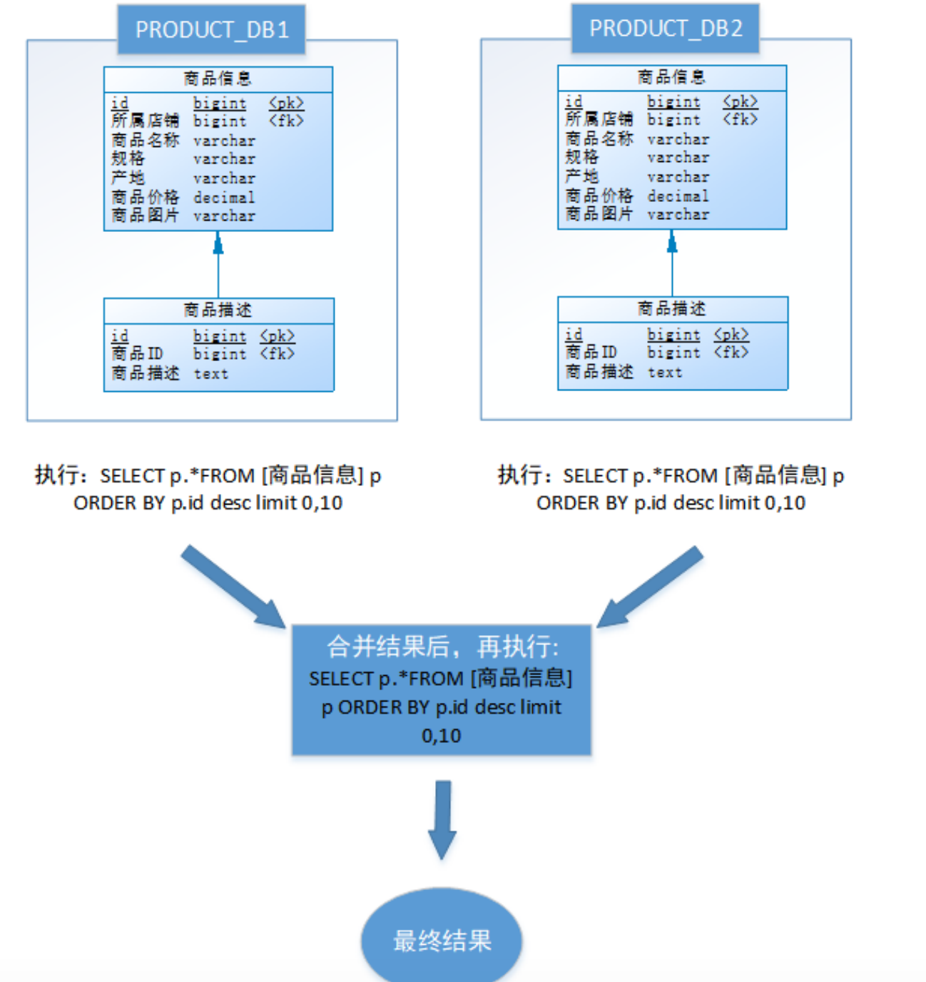
The above process is to take the data of the first page, which has little impact on the performance. However, due to the distribution of commodity information, the data in each database may be random. If you take page n, you need to take out and merge the data of the first N pages of all nodes, and then sort them as a whole. The operation efficiency can be imagined. Therefore, the larger the number of requested pages, the worse the performance of the system will be. When using functions such as Max, Min, Sum and Count for calculation, just like sorting and paging, you also need to execute the corresponding functions on each partition first, then summarize and recalculate the result set of each partition, and finally return the result.

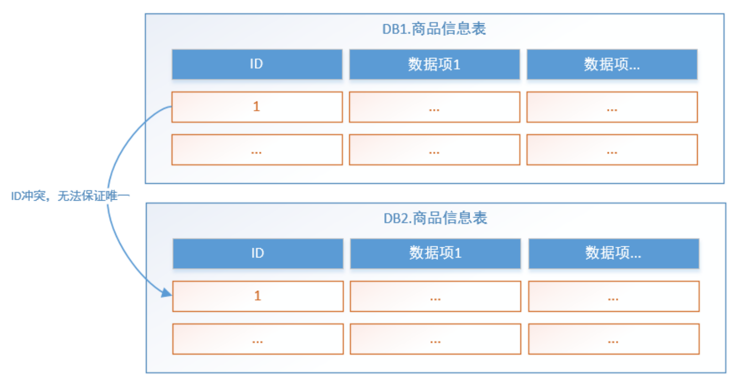
1.3.4 weight avoidance

In the sub database and sub table environment, since the data in the table exists in different databases at the same time, the self growth of the primary key value usually used will be useless, and the ID generated by a partitioned database cannot be guaranteed to be globally unique. Therefore, the global primary key needs to be designed separately to avoid the duplication of cross database primary keys.

1.3.5 public table

In practical application scenarios, parameter tables and data dictionary tables are dependency tables with small amount of data and little change, and belong to high-frequency joint query. The geographic region table in the example also belongs to this type.

You can save a copy of this kind of table in each database, and all updates to the public table are sent to all sub databases for execution at the same time.

After the database and table are divided, the data is scattered in different databases and servers. Therefore, the operation of data can not be completed in the conventional way, and it also brings a series of problems. Fortunately, not all of these problems need to be solved at the application level. There are many middleware on the market for us to choose from, among which sharding JDBC is popular. Let's learn about it.

1.4 sharding JDBC introduction

1.4.1 sharding JDBC introduction

Sharding JDBC is an open source distributed database middleware developed by Dangdang. Sharding JDBC has been included in sharding sphere since 3.0, and then the project enters the Apache incubator. The version after version 4.0 is the Apache version.

ShardingSphere is an ecosystem composed of a set of open-source distributed database middleware solutions. It is composed of three independent products: sharding JDBC, ShardingProxy and sharding sidecar (planned). They all provide standardized data fragmentation, distributed transaction and database governance functions, which can be applied to various application scenarios such as Java isomorphism, heterogeneous language, container, cloud native and so on.

Official address: https://shardingsphere.apache.org/document/current/cn/overview/

At present, we only need to focus on sharding JDBC, which is positioned as a lightweight Java framework and provides additional services in the JDBC layer of Java. It uses the client to connect directly to the database and provides services in the form of jar package without additional deployment and dependence. It can be understood as an enhanced version of JDBC Driver and is fully compatible with JDBC and various ORM frameworks.

The core function of sharding jdbc is data fragmentation and read-write separation. Through sharding jdbc, applications can use jdbc to access multiple data sources that have been divided into databases, tables and read-write separation transparently, without caring about the number of data sources and how the data is distributed.

1. It is applicable to any ORM framework based on Java, such as Hibernate, Mybatis, Spring JDBC Template or directly using JDBC.
2. Database connection pool based on any third party, such as DBCP, C3P0, BoneCP, Druid, HikariCP, etc. Support any database that implements JDBC specification.
3. At present, MySQL, Oracle, SQLServer and PostgreSQL are supported.

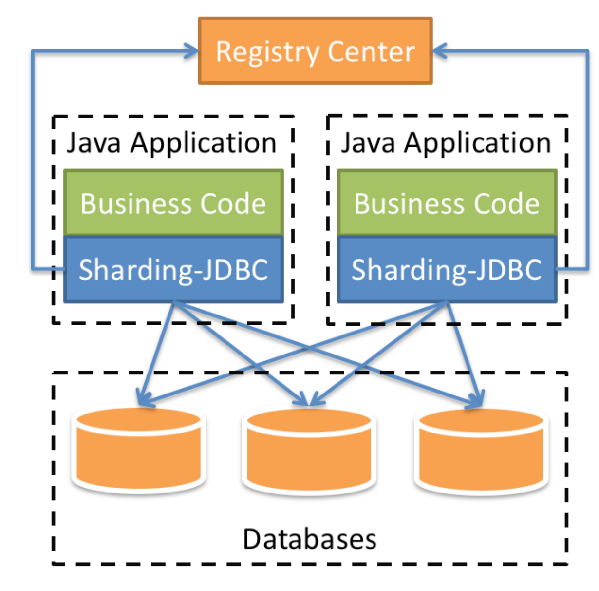
The above figure shows the working mode of sharding Jdbc. Before using sharding Jdbc, the database needs to be divided into databases and tables manually, and the Jar package of sharding Jdbc is added to the application. The application operates the database and data tables after dividing databases and tables through sharding Jdbc. Because sharding Jdbc is an enhancement of the Jdbc driver, using sharding Jdbc is like using the Jdbc driver, There is no need to specify the specific sub database and sub table to be operated in the application.

1.4.2 performance comparison with jdbc

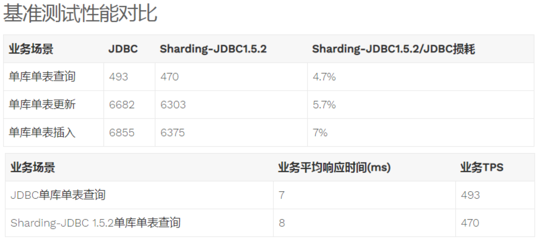
1. Performance loss test: the server resources are sufficient and the concurrency number is the same. Compare the performance loss of JDBC and sharding JDBC, and the loss of sharding JDBC relative to JDBC is no more than 7%.
   

2. Performance comparison test: server resources are used to the limit, and the throughput of JDBC and sharding JDBC in the same scenario is equivalent.

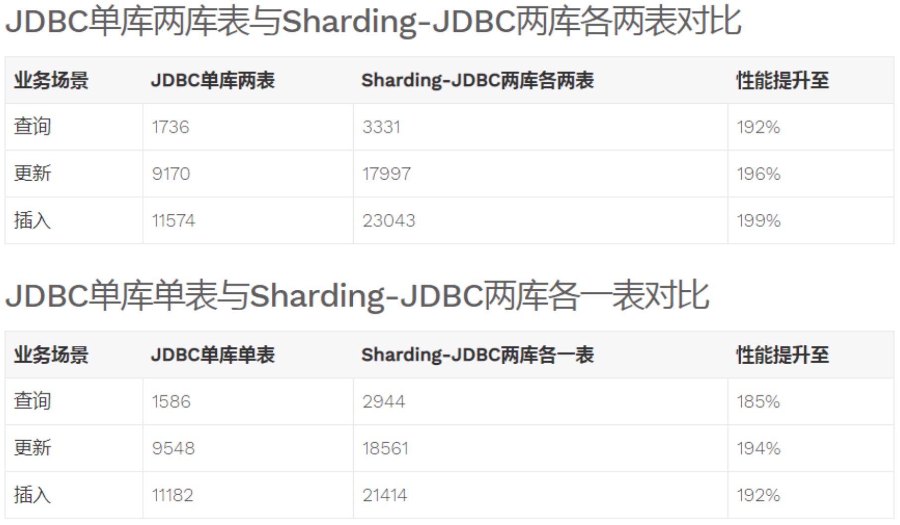
3. Performance comparison test: the server resources are used to the limit. After sharding JDBC adopts sub database and sub table, the throughput of sharding JDBC is nearly twice that of JDBC without sub table.
   

2 sharding JDBC quick start

2.1 requirements description

This chapter uses sharding JDBC to complete the horizontal division of the order table, and quickly experience the use of sharding JDBC through the development of quick start program.

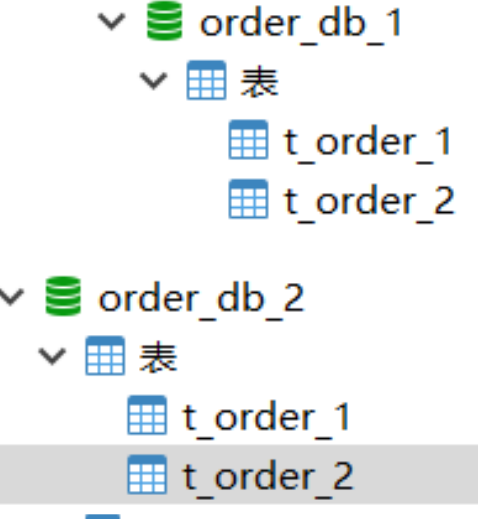
Create two tables manually, t_order_1 and t_order_2. These two tables are the tables after the order table is split. Insert data into the order table through sharding JDBC. According to certain fragmentation rules, enter t with even primary key_ order_ 1. Another part of data enters t_order_2. Query the data through sharding JDBC, and start from t according to the content of SQL statement_ order_ 1 or t_order_2. Query data.

2.2 environment construction

2.2.1 environmental description

Operating system: Win10
Database: MySQL-5.7.25
JDK: 64 bit jdk1 8.0_ two hundred and one
Application framework: spring-boot-2.1.3 RELEASE，Mybatis3. five
Sharding-JDBC: sharding-jdbc-spring-boot-starter-4.0.0-RC1

2.2.2 creating database

#Create order library order_db

CREATE DATABASE `order_db` CHARACTER SET 'utf8' COLLATE 'utf8_general_ci';

In order_ Create t in DB_ order_ 1,t_ order_ Table 2

DROP TABLE IF EXISTS `t_order_1`;
CREATE TABLE `t_order_1` (
`order_id` bigint(20) NOT NULL COMMENT 'order id',
`price` decimal(10, 2) NOT NULL COMMENT 'Order price',
`user_id` bigint(20) NOT NULL COMMENT 'Order user id',
`status` varchar(50) CHARACTER SET utf8 COLLATE utf8_general_ci NOT NULL COMMENT 'Order status',
PRIMARY KEY (`order_id`) USING BTREE
) ENGINE = InnoDB CHARACTER SET = utf8 COLLATE = utf8_general_ci ROW_FORMAT = Dynamic;

DROP TABLE IF EXISTS `t_order_2`;
CREATE TABLE `t_order_2` (
`order_id` bigint(20) NOT NULL COMMENT 'order id',
`price` decimal(10, 2) NOT NULL COMMENT 'Order price',
`user_id` bigint(20) NOT NULL COMMENT 'Order user id',
`status` varchar(50) CHARACTER SET utf8 COLLATE utf8_general_ci NOT NULL COMMENT 'Order status',
PRIMARY KEY (`order_id`) USING BTREE
) ENGINE = InnoDB CHARACTER SET = utf8 COLLATE = utf8_general_ci ROW_FORMAT = Dynamic;

2.2.3 introducing maven dependency

Jar package integrating sharding JDBC and SpringBoot is introduced:

<dependency>
  <groupId>org.apache.shardingsphere</groupId>
  <artifactId>sharding‐jdbc‐spring‐boot‐starter</artifactId>
  <version>4.0.0‐RC1</version>
</dependency>

Please refer to the dbsharding / sharding JDBC simple project in resources for specific spring boot dependencies and configurations. This guide only describes the contents related to sharding JDBC.

2.3 programming

2.3.1 partition rule configuration

Sharding rule configuration is an important basis for sharding JDBC to perform database and table operations. The configuration contents include: data source, primary key generation strategy, sharding strategy, etc.

In application Configuration in properties

server.port=56081

spring.application.name = sharding-jdbc-simple-demo

server.servlet.context-path = /sharding-jdbc-simple-demo
spring.http.encoding.enabled = true
spring.http.encoding.charset = UTF-8
spring.http.encoding.force = true

#Duplicate bean definition override
spring.main.allow-bean-definition-overriding = true
#
mybatis.configuration.map-underscore-to-camel-case = true

#Sharding JDBC sharding rule configuration
#data source
spring.shardingsphere.datasource.names = m1

spring.shardingsphere.datasource.m1.type = com.alibaba.druid.pool.DruidDataSource
spring.shardingsphere.datasource.m1.driver-class-name = com.mysql.jdbc.Driver
spring.shardingsphere.datasource.m1.url = jdbc:mysql://localhost:3306/order_db?useUnicode=true
spring.shardingsphere.datasource.m1.username = root
spring.shardingsphere.datasource.m1.password = 123456

# Specify t_ For the data distribution of the order table, configure the data node M1 t_order_ 1,m1. t_order_ two
spring.shardingsphere.sharding.tables.t_order.actual-data-nodes = m1.t_order_$->{1..2}

# Specify t_ The primary key generation strategy of order table is SNOWFLAKE
spring.shardingsphere.sharding.tables.t_order.key-generator.column=order_id
spring.shardingsphere.sharding.tables.t_order.key-generator.type=SNOWFLAKE

# Specify t_ The order slicing strategy includes the key slicing strategy and the table slicing strategy
spring.shardingsphere.sharding.tables.t_order.table-strategy.inline.sharding-column = order_id
spring.shardingsphere.sharding.tables.t_order.table-strategy.inline.algorithm-expression = t_order_$->{order_id % 2 + 1}

# Open sql output log
spring.shardingsphere.props.sql.show = true

swagger.enable = true

logging.level.root = info
logging.level.org.springframework.web = info
logging.level.com.itheima.dbsharding  = debug
logging.level.druid.sql = debug

1. First, define the data source m1 and configure the actual parameters of m1.
2. Specify t_ Data distribution of order table, which is distributed in M1 t_order_ 1，m1. t_order_ two
3. Specify t_ The primary key generation strategy of order table is SNOWFLAKE. SNOWFLAKE is a distributed self increasing algorithm to ensure the global uniqueness of id
4. Definition t_order fragmentation strategy_ Data with even ID falls in t_order_1. The odd number falls on t_order_2. The expression of table splitting strategy is t_order_$-> {order_id % 2 + 1}

2.3.2 data operation

@Mapper
@Component
public interface OrderDao {
    /**
    * New order
    * @param price Order price
    * @param userId User id
    * @param status Order status
    * @return
    */
    @Insert("insert into t_order(price,user_id,status) value(#{price},#{userId},#{status})")
    int insertOrder(@Param("price") BigDecimal price, @Param("userId")Long userId,
    @Param("status")String status);
    /**
    * Query multiple orders by id list
    * @param orderIds Order id list
    * @return
    */
    @Select({"<script>" +
    "select " +
    " * " +
    " from t_order t" +
    " where t.order_id in " +
    "<foreach collection='orderIds' item='id' open='(' separator=',' close=')'>" +
    " #{id} " +
    "</foreach>"+
    "</script>"})
    List<Map> selectOrderbyIds(@Param("orderIds")List<Long> orderIds);
}

2.3.3 testing

Write unit tests:
@RunWith(SpringRunner.class)
@SpringBootTest(classes = {ShardingJdbcSimpleDemoBootstrap.class})
public class OrderDaoTest {
    @Autowired
    private OrderDao orderDao;
    @Test
    public void testInsertOrder(){
        for (int i = 0 ; i<10; i++){
            orderDao.insertOrder(new BigDecimal((i+1)*5),1L,"WAIT_PAY");
        }
    }


    @Test
    public void testSelectOrderbyIds(){
        List<Long> ids = new ArrayList<>();
        ids.add(373771636085620736L);
        ids.add(373771635804602369L);
        List<Map> maps = orderDao.selectOrderbyIds(ids);
        System.out.println(maps);
    }
}

Execute testInsertOrder:

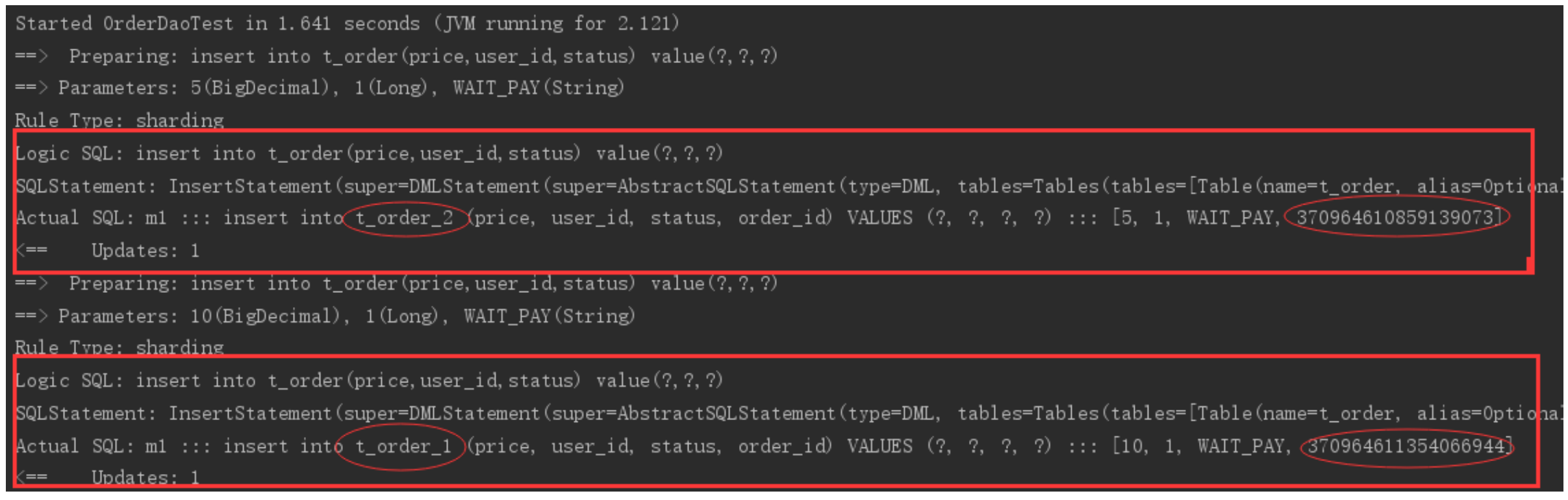
Order can be found through the log_ Odd ID is inserted into t_ order_ Table 2, even numbers are inserted into t_order_1 table to achieve the expected objectives.

Execute testSelectOrderbyIds:

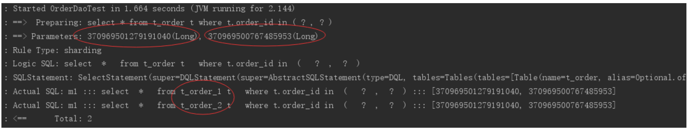
Through the log, it can be found that according to the incoming order_ The parity of IDS is different. Sharding JDBC retrieves data from different tables to achieve the desired goal.

2.4 process analysis

Through log analysis, what did sharding JDBC do after getting the sql to be executed by the user:

1. Parse the sql to obtain the slice key value, in this case, order_id
2. Sharding JDBC configures T through rules_ order_$-> {order_id% 2 + 1}, OK, when order_ When the ID is even, it should go to t_order_1. Insert the data in the table. When it is an odd number, go to t_order_2 insert data.
3. So sharding JDBC according to order_ The ID of the SQL statement to be rewritten is the actual value of the SQL statement to be executed.
4. Execute the rewritten real sql statement
5. Summarize and merge all the actual sql execution results and return.

2.5 other integration methods

Sharding JDBC can not only integrate well with spring boot, but also support other configuration methods. It supports the following four integration methods.

Spring Boot Yaml configuration definition application YML, as follows:

server:
  port: 56081
  servlet:
    context-path: /sharding-jdbc-simple-demo
spring:
  application:
    name: sharding-jdbc-simple-demo
  http:
    encoding:
      enabled: true
      charset: utf-8
      force: true
  main:
    allow-bean-definition-overriding: true
  shardingsphere:
    datasource:
      names: m1
      m1:
        type: com.alibaba.druid.pool.DruidDataSource
        driverClassName: com.mysql.jdbc.Driver
        url: jdbc:mysql://localhost:3306/order_db?useUnicode=true
        username: root
        password: 123456
    sharding:
      tables:
        t_order:
          actualDataNodes: m1.t_order_$->{1..2}
          tableStrategy:
            inline:
              shardingColumn: order_id
              algorithmExpression: t_order_$->{order_id % 2 + 1}
          keyGenerator:
            type: SNOWFLAKE
            column: order_id
    props:
      sql:
        show: true
mybatis:
  configuration:
    map-underscore-to-camel-case: true
swagger:
  enable: true
logging:
  level:
    root: info
    org.springframework.web: info
    com.itheima.dbsharding: debug
    druid.sql: debug

If using application YML needs to mask the original application Properties file.

Add configuration class to Java configuration:

package com.itheima.dbsharding.simple.config;

import com.alibaba.druid.pool.DruidDataSource;
import org.apache.shardingsphere.api.config.sharding.KeyGeneratorConfiguration;
import org.apache.shardingsphere.api.config.sharding.ShardingRuleConfiguration;
import org.apache.shardingsphere.api.config.sharding.TableRuleConfiguration;
import org.apache.shardingsphere.api.config.sharding.strategy.InlineShardingStrategyConfiguration;
import org.apache.shardingsphere.shardingjdbc.api.ShardingDataSourceFactory;
import org.springframework.context.annotation.Bean;

import javax.sql.DataSource;
import java.sql.SQLException;
import java.util.HashMap;
import java.util.Map;
import java.util.Properties;

/**
 * Code mode configuration
 *
 * @author bcl
 * @date 2022/2/18
 */
//@Configuration
public class ShardingJdbcConfig {

    //Configure fragmentation rules
    // Define data source
    Map<String, DataSource> createDataSourceMap() {
        DruidDataSource dataSource1 = new DruidDataSource();
        dataSource1.setDriverClassName("com.mysql.jdbc.Driver");
        dataSource1.setUrl("jdbc:mysql://localhost:3306/order_db?useUnicode=true");
        dataSource1.setUsername("root");
        dataSource1.setPassword("123456");
        Map<String, DataSource> result = new HashMap<>();
        result.put("m1", dataSource1);
        return result;
    }

    // Define primary key generation policy
    private static KeyGeneratorConfiguration getKeyGeneratorConfiguration() {
        KeyGeneratorConfiguration result = new KeyGeneratorConfiguration("SNOWFLAKE", "order_id");
        return result;
    }

    // Definition t_ Sharding strategy of order table
    TableRuleConfiguration getOrderTableRuleConfiguration() {
        TableRuleConfiguration result = new TableRuleConfiguration("t_order", "m1.t_order_$->{1..2}");
        result.setTableShardingStrategyConfig(new InlineShardingStrategyConfiguration("order_id", "t_order_$->{order_id % 2 + 1}"));
        result.setKeyGeneratorConfig(getKeyGeneratorConfiguration());

        return result;
    }

    // Defining sharding JDBC data sources
    @Bean
    DataSource getShardingDataSource() throws SQLException {
        ShardingRuleConfiguration shardingRuleConfig = new ShardingRuleConfiguration();
        shardingRuleConfig.getTableRuleConfigs().add(getOrderTableRuleConfiguration());
        //spring.shardingsphere.props.sql.show = true
        Properties properties = new Properties();
        properties.put("sql.show", "true");
        return ShardingDataSourceFactory.createDataSource(createDataSourceMap(), shardingRuleConfig, properties);
    }

}

Because the configuration class is adopted, the original application needs to be shielded Spring. In the properties file Configuration information starting with shardingsphere. You also need to mask the use of spring. Com in the SpringBoot startup class Class of shardingsphere configuration item:

@SpringBootApplication(exclude = {SpringBootConfiguration.class}) 
public class ShardingJdbcSimpleDemoBootstrap {....}

Spring Boot properties is configured in the same way as the quick start program.

#Sharding JDBC sharding rule configuration
#Define data source
spring.shardingsphere.datasource.names = m1

spring.shardingsphere.datasource.m1.type = com.alibaba.druid.pool.DruidDataSource
spring.shardingsphere.datasource.m1.driver-class-name = com.mysql.jdbc.Driver
spring.shardingsphere.datasource.m1.url = jdbc:mysql://localhost:3306/order_db?useUnicode=true
spring.shardingsphere.datasource.m1.username = root
spring.shardingsphere.datasource.m1.password = 123456

# Specify t_ For the data distribution of the order table, configure the data node M1 t_order_ 1,m1. t_order_ two
spring.shardingsphere.sharding.tables.t_order.actual-data-nodes = m1.t_order_$->{1..2}

# Specify t_ The primary key generation strategy of order table is SNOWFLAKE
spring.shardingsphere.sharding.tables.t_order.key-generator.column=order_id
spring.shardingsphere.sharding.tables.t_order.key-generator.type=SNOWFLAKE

# Specify t_ The order slicing strategy includes the key slicing strategy and the table slicing strategy
spring.shardingsphere.sharding.tables.t_order.table-strategy.inline.sharding-column = order_id
spring.shardingsphere.sharding.tables.t_order.table-strategy.inline.algorithm-expression = t_order_$->{order_id % 2 + 1}

Spring namespace configuration this method uses xml configuration, which is not recommended.

<?xml version="1.0" encoding="UTF‐8"?>
<beans xmlns="http://www.springframework.org/schema/beans"
xmlns:xsi="http://www.w3.org/2001/XMLSchema‐instance"
xmlns:p="http://www.springframework.org/schema/p"
xmlns:context="http://www.springframework.org/schema/context"
xmlns:tx="http://www.springframework.org/schema/tx"
xmlns:sharding="http://shardingsphere.apache.org/schema/shardingsphere/sharding"

xsi:schemaLocation="http://www.springframework.org/schema/beans
http://www.springframework.org/schema/beans/spring‐beans.xsd
http://shardingsphere.apache.org/schema/shardingsphere/sharding
http://shardingsphere.apache.org/schema/shardingsphere/sharding/sharding.xsd
http://www.springframework.org/schema/context
http://www.springframework.org/schema/context/spring‐context.xsd
http://www.springframework.org/schema/tx
http://www.springframework.org/schema/tx/spring‐tx.xsd">
    <context:annotation‐config />
    <!‐‐Define multiple data sources‐‐>
    <bean id="m1" class="com.alibaba.druid.pool.DruidDataSource" destroy‐method="close">
        <property name="driverClassName" value="com.mysql.jdbc.Driver" />
        <property name="url" value="jdbc:mysql://localhost:3306/order_db_1?useUnicode=true" />
        <property name="username" value="root" />
        <property name="password" value="root" />
    </bean>
    <!‐‐Define sub database policy‐‐>
    <sharding:inline‐strategy id="tableShardingStrategy" sharding‐column="order_id" algorithm‐
    expression="t_order_$‐>{order_id % 2 + 1}" />
    <!‐‐Define primary key generation policy‐‐>
    <sharding:key‐generator id="orderKeyGenerator" type="SNOWFLAKE" column="order_id" />
    <!‐‐definition sharding‐Jdbc data source‐‐>
    <sharding:data‐source id="shardingDataSource">
        <sharding:sharding‐rule data‐source‐names="m1">
            <sharding:table‐rules>
                <sharding:table‐rule logic‐table="t_order" table‐strategy‐ref="tableShardingStrategy" key‐generator‐ref="orderKeyGenerator" />
            </sharding:table‐rules>
        </sharding:sharding‐rule>
    </sharding:data‐source>
</beans>

3 sharding JDBC execution principle

3.1 basic concepts

Before understanding the execution principle of sharding JDBC, you need to understand the following concepts:

1. Logic table
   The general name of a horizontally split data table. Example: the order data table is divided into 10 tables according to the mantissa of the primary key, which are t_order_0 , t_order_1 to t_order_9. Their logical table is named t_order .

2. Real table
   A physical table that exists in a fragmented database. T in the previous example_ order_ 0 to t_order_9. Data node is the smallest physical unit of data fragmentation. It is composed of data source name and data table, for example: ds_0.t_order_0

3. Binding table
   It refers to the main table and sub table with consistent fragmentation rules. For example: t_order table and t_order_item table, all according to order_id fragmentation, and the partition keys between bound tables are exactly the same, then the two tables are bound to each other. The Cartesian product association will not appear in the multi table Association query between bound tables, and the efficiency of association query will be greatly improved. For example, if the SQL is:

   SELECT i.* FROM t_order o JOIN t_order_item i ON o.order_id=i.order_id WHERE o.order_id in (10,11);
   

   When the binding table relationship is not configured, the sharding key order is assumed_ ID route the value 10 to slice 0 and the value 11 to slice 1, then the SQL after routing should be 4, which are presented as Cartesian Products:

   SELECT i.* FROM t_order_0 o JOIN t_order_item_0 i ON o.order_id=i.order_id WHERE o.order_id in (10, 11);
   SELECT i.* FROM t_order_0 o JOIN t_order_item_1 i ON o.order_id=i.order_id WHERE o.order_id in (10, 11);
   SELECT i.* FROM t_order_1 o JOIN t_order_item_0 i ON o.order_id=i.order_id WHERE o.order_id in (10, 11);
   SELECT i.* FROM t_order_1 o JOIN t_order_item_1 i ON o.order_id=i.order_id WHERE o.order_id in (10, 11);
   

   After configuring the binding table relationship, the route SQL should be 2:

   SELECT i.* FROM t_order_0 o JOIN t_order_item_0 i ON o.order_id=i.order_id WHERE o.order_id in (10, 11);
   SELECT i.* FROM t_order_1 o JOIN t_order_item_1 i ON o.order_id=i.order_id WHERE o.order_id in (10, 11);
   

4. Broadcast table
   It refers to the table existing in all fragment data sources. The table structure and the data in the table are completely consistent in each database. It is applicable to scenarios where the amount of data is small and needs to be associated with tables with massive data, such as dictionary tables.

5. Slice key
   The database field used for fragmentation is the key field to split the database (table) horizontally. For example, if the mantissa of the order primary key in the order table is taken as modular fragment, the order primary key is a fragment field. If there is no fragment field in SQL, full routing will be executed and the performance is poor. In addition to the support of single sharding field, ShardingJdbc also supports sharding according to multiple fields.

6. Partition algorithm
   It includes partition key and partition algorithm. Due to the independence of partition algorithm, it is separated independently. What can be used for sharding operation is sharding key + sharding algorithm, that is, sharding strategy. The built-in fragmentation strategy can be roughly divided into mantissa modulus, hash, range, label, time, etc. The slicing strategy configured by the user side is more flexible. The commonly used line expression is used to configure the slicing strategy, which is expressed by Groovy expression, such as: t_user_$-> {u_id% 8} indicates t_user table according to u_ ID module 8 is divided into 8 tables, and the table name is t_user_0 to t_user_7 .

7. Auto increment primary key generation strategy
   By generating self incrementing primary keys on the client to replace the original self incrementing primary keys of the database, there is no duplication of distributed primary keys.

3.2 SQL parsing

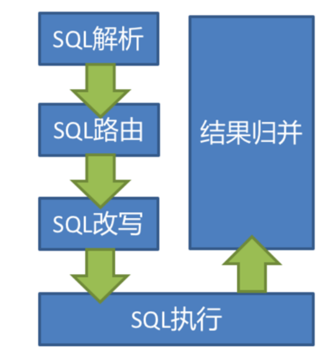
When sharding JDBC receives an SQL statement, it will execute one after another
SQL parsing = > query optimization = > sql routing = > sql rewriting = > sql execution = > result merging,
Finally, the execution result is returned.

SQL parsing process is divided into lexical parsing and syntax parsing. Lexical parser is used to disassemble SQL into non separable atomic symbols, which is called Token. According to the dictionaries provided by different database dialects, they are classified into keywords, expressions, literals and operators. Then use the syntax parser to convert the SQL into an abstract syntax tree.
For example, the following SQL:

SELECT id, name FROM t_user WHERE status = 'ACTIVE' AND age > 18

The parsed is an abstract syntax tree, as shown in the following figure:

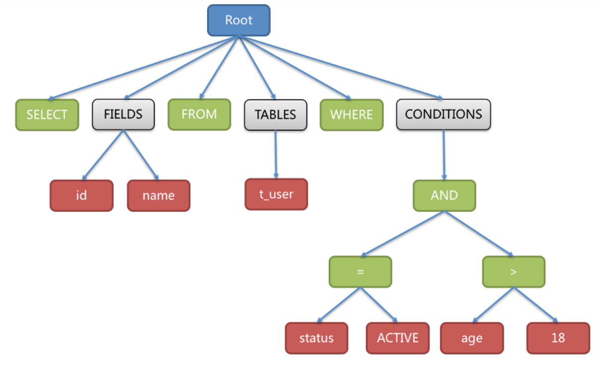
In order to facilitate understanding, the Token of the keyword in the abstract syntax tree is represented in green, the Token of the variable is represented in red, and the gray indicates that it needs to be further split.

Finally, through the traversal of the abstract syntax tree, the context required for segmentation is refined, and the location where SQL rewriting (described later) may be required is marked. The parsing context for sharding includes query selection items, Table information, Sharding Condition, Auto increment Primary Key, Order By, Group By, and page information (Limit, Rownum, Top).

3.3 SQL routing

SQL routing is the process of mapping data operations on logical tables to operations on data nodes. Match the partition strategy of database and table according to the parsing context, and generate the routing path. SQL with fragment key can be divided into single chip routing (the operator of fragment key is equal sign), multi chip routing (the operator of fragment key is IN) and range routing (the operator of fragment key is BETWEEN). SQL without fragment key adopts broadcast routing. The scenarios of routing based on fragment keys can be divided into direct routing, standard routing, Cartesian routing, etc.

1. Standard routing
   Standard routing is sharding JDBC's most recommended fragmentation method. Its scope of application is SQL that does not contain Association queries or only contains Association queries BETWEEN bound tables. When the fragment operator is equal sign, the routing result will fall into a single database (table). When the fragment operator is BETWEEN or IN, the routing result may not fall into a unique database (table). Therefore, a logical SQL may eventually be split into multiple real SQL for execution. For example, if you follow order_ The odd and even numbers of ID are used for data fragmentation. The SQL of a single table query is as follows:

   SELECT * FROM t_order WHERE order_id IN (1, 2);
   

   Then the result of routing should be:

   SELECT * FROM t_order_0 WHERE order_id IN (1, 2);
   SELECT * FROM t_order_1 WHERE order_id IN (1, 2);
   

   The complexity and performance of associated queries of bound tables are equivalent to those of single table queries. For example, if the SQL of an associated query containing a bound table is as follows:

   SELECT * FROM t_order o JOIN t_order_item i ON o.order_id=i.order_id WHERE order_id IN (1, 2);
   

   Then the result of routing should be:

   SELECT * FROM t_order_0 o JOIN t_order_item_0 i ON o.order_id=i.order_id WHERE order_id IN (1,2);
   SELECT * FROM t_order_1 o JOIN t_order_item_1 i ON o.order_id=i.order_id WHERE order_id IN (1,2);
   

   You can see that the number of SQL splits is consistent with that of a single table.

2. Cartesian routing
   Cartesian routing is the most complex case. It cannot locate the fragmentation rules according to the relationship between bound tables. Therefore, the association query between unbound tables needs to be disassembled into Cartesian product combination for execution. If the SQL in the previous example does not configure the binding table relationship, the result of the route should be:

   SELECT * FROM t_order_0 o JOIN t_order_item_0 i ON o.order_id=i.order_id WHERE order_id IN (1,2);
   SELECT * FROM t_order_0 o JOIN t_order_item_1 i ON o.order_id=i.order_id WHERE order_id IN (1,2);
   SELECT * FROM t_order_1 o JOIN t_order_item_0 i ON o.order_id=i.order_id WHERE order_id IN (1,2);
   SELECT * FROM t_order_1 o JOIN t_order_item_1 i ON o.order_id=i.order_id WHERE order_id IN (1,2);
   

   Cartesian routing query has low performance and should be used with caution.

3. Full database table routing
   For SQL without fragment key, broadcast routing is adopted. According to the SQL type, it can be divided into five types: full database table routing, full database routing, full instance routing, unicast routing and blocking routing. The full database table routing is used to handle the operation of all real tables related to their logical tables in the database, mainly including DQL (data query) and DML (data manipulation) without fragment key, DDL (data definition), etc. For example:

   SELECT * FROM t_order WHERE good_prority IN (1, 10);
   

   It will traverse all tables in all databases, match the logical table and the real table name one by one, and execute if it can match. Become after routing

   SELECT * FROM t_order_0 WHERE good_prority IN (1, 10);
   SELECT * FROM t_order_1 WHERE good_prority IN (1, 10);
   SELECT * FROM t_order_2 WHERE good_prority IN (1, 10);
   SELECT * FROM t_order_3 WHERE good_prority IN (1, 10);
   

3.4 SQL rewriting

The SQL written by engineers for logical tables cannot be directly executed in the real database. SQL rewriting is used to rewrite logical SQL into SQL that can be correctly executed in the real database.
As a simple example, if the logical SQL is:

SELECT order_id FROM t_order WHERE order_id=1;

Suppose that the SQL is configured with the sharding key order_id and order_ If id = 1, it will be routed to fragment Table 1. The rewritten SQL should be:

SELECT order_id FROM t_order_1 WHERE order_id=1;

For another example, sharding JDBC needs to obtain the corresponding data when merging the results, but the data cannot be returned through the SQL query. This situation is mainly for GROUP BY and ORDER BY. When merging results, you need to group and sort according to the field items of GROUP BY and ORDER BY. However, if the selection items of the original SQL do not contain grouping items or sorting items, you need to rewrite the original SQL. Let's take a look at the scenario in the original SQL with the information required for result merging:

SELECT order_id, user_id FROM t_order ORDER BY user_id;

Due to the use of user_id to sort. In the result merging, you need to be able to get the user_id, and the above SQL can get user_id data, so there is no need to add columns. If the selected item does not contain the columns required for result merging, supplementary columns are required, such as the following SQL:

SELECT order_id FROM t_order ORDER BY user_id;

Because the original SQL does not contain the user that needs to be obtained in the result merging_ ID, so the SQL needs to be supplemented and rewritten. The SQL after column supplement is:

SELECT order_id, user_id AS ORDER_BY_DERIVED_0 FROM t_order ORDER BY user_id;

3.5 SQL execution

Sharding JDBC adopts a set of automatic execution engine, which is responsible for sending the real SQL after routing and rewriting safely and efficiently to the underlying data source for execution. It does not simply send SQL directly to the data source through JDBC for execution; Nor does it directly put the execution request into the thread pool for concurrent execution. It pays more attention to balancing the consumption caused by data source connection creation and memory occupation, as well as maximizing the rational use of concurrency. The goal of the execution engine is to automatically balance resource control and execution efficiency. It can adaptively switch between the following two modes:

1. Memory limit mode
   The premise of using this mode is that sharding JDBC does not limit the number of database connections consumed by one operation. If the actual SQL needs to operate on 200 tables in a database instance, create a new database connection for each table and process it concurrently through multithreading to maximize the execution efficiency.

2. Connection restriction mode
   The premise of using this mode is that sharding JDBC strictly controls the number of database connections consumed in one operation. If the actually executed SQL needs to operate on 200 tables in a database instance, only a unique database connection will be created and its 200 tables will be processed serially. If the fragments in one operation are scattered in different databases, multithreading is still used to handle the operations on different libraries, but each operation of each library still creates only one unique database connection.

3. The memory restriction mode is applicable to OLAP operation, which can improve the system throughput by relaxing the restrictions on database connection; The connection restriction mode is applicable to OLTP operation. OLTP usually has a partition key and will be routed to a single partition. Therefore, it is a wise choice to strictly control the database connection to ensure that the online system database resources can be used by more applications.

3.6 result merging

Combining multiple data result sets obtained from various data nodes into one result set and returning them to the requesting client correctly is called result merging. The result merging supported by sharding JDBC can be divided into five types: traversal, sorting, grouping, paging and aggregation. They are combined rather than mutually exclusive. Merge engine
The overall structure is divided as follows.

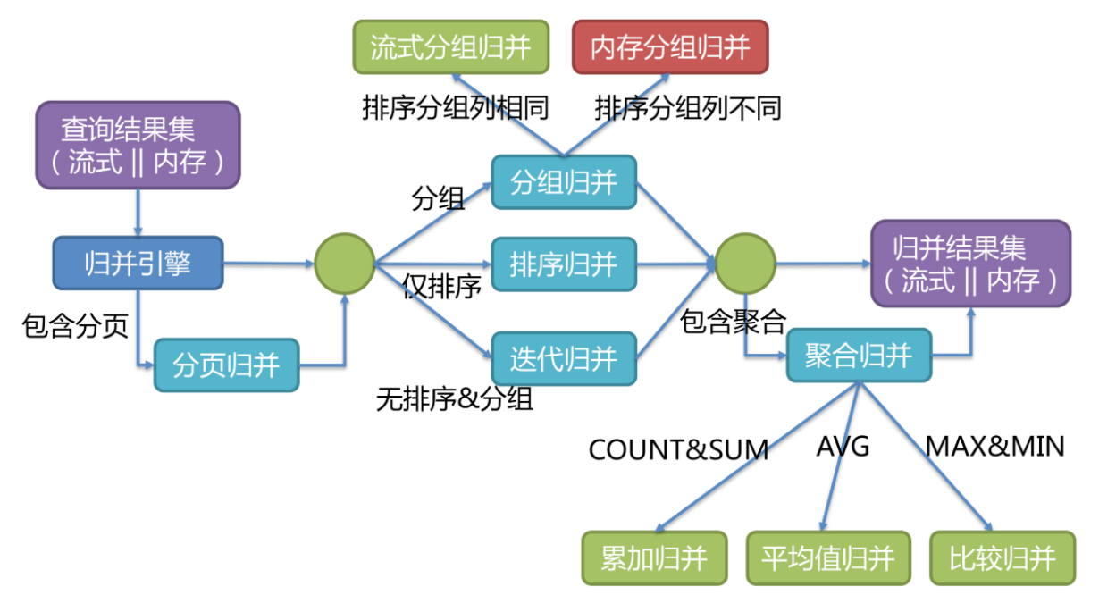
Results merging can be divided into flow merging, memory merging and decorator merging. Stream merge and memory merge are mutually exclusive. Decorator merge can do further processing on stream merge and memory merge.

Memory merging is easy to understand. It traverses and stores the data of all fragment result sets in memory, and then encapsulates them into an item by item access data result set after unified grouping, sorting, aggregation and other calculations.

Stream merging means that every time the data obtained from the database result set can return the correct single piece of data one by one through the cursor. It is most consistent with the original way of returning the result set of the database.

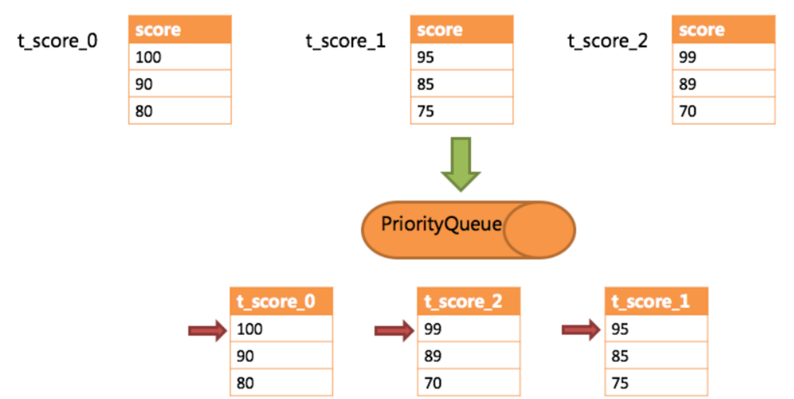
The following is an example to illustrate the process of sorting and merging. As shown in the figure below, it is an example of sorting by score, which adopts the flow merging method. The figure shows the data result sets returned from three tables. Each data result set has been sorted according to the score, but the three data result sets are out of order. Sort the data values pointed to by the current cursor of the three data result sets and put them into the priority queue, t_ score_ The first data value of 0 is the largest, t_ score_ The first data value of 2 takes the second place, t_ score_ The first data value of 1 is the smallest, so the priority queue is based on t_score_0，t_score_2 and t_score_1 to sort the queue.

The following figure shows how sorting and merging are carried out when calling next. From the figure, we can see that when the next call is made for the first time, t is at the top of the queue_ score_ 0 will be ejected from the queue, and the data value pointed by the current cursor (i.e. 100) will be returned to the query client. After moving the cursor down one bit, it will be put back into the priority queue. The priority queue will also be based on t_ score_ The current data result set of 0 points to the data value of the cursor (here is 90) for sorting. According to the current value, t_score_0 is ranked last in the queue. The second t in the previous queue_ score_ The data result set of 2 automatically ranks first in the queue.

In the second next, you only need to put the t that is currently at the top of the queue_ score_ 2 pop up the queue, return the value pointed to by the data result set cursor to the client, move the cursor down, continue to join the queue, and so on. When there is no data in a result set, there is no need to join the queue again

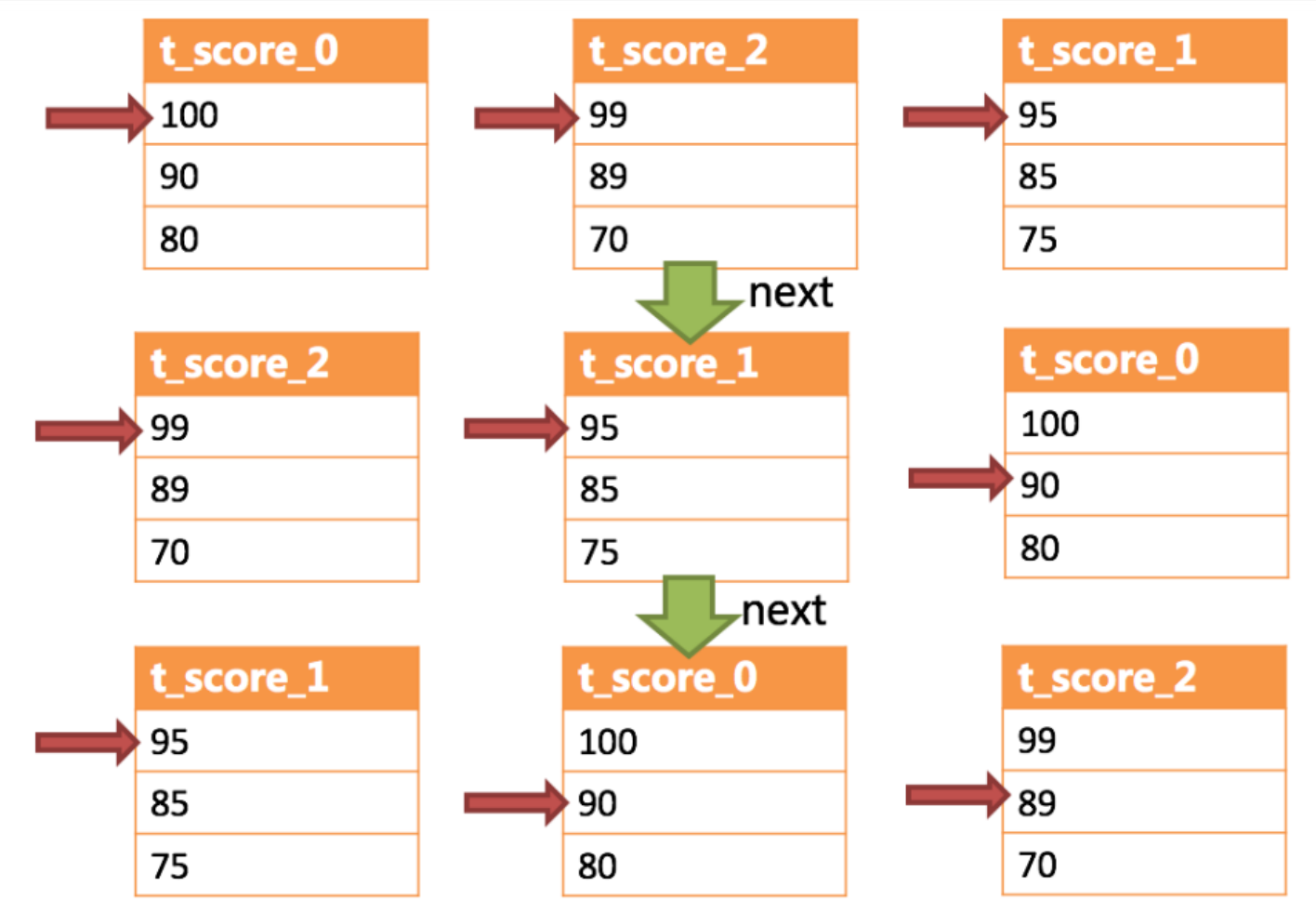
It can be seen that when the data in each data result set is orderly and the multi data result set is disordered as a whole, sharding JDBC does not need to load all the data into memory to sort. It uses the method of stream merging, and only one correct piece of data is obtained each time next, which greatly saves the consumption of memory.

Decorator merging is a unified function enhancement for the merging of all result sets. For example, before the SUM needs to be aggregated during merging, the result set will be queried through memory merging or streaming merging before aggregation calculation. Therefore, aggregation merging is a merging ability added to the merging type introduced earlier, that is, decorator mode.

3.7 summary

Through the above introduction, I believe you have understood the basic concept, core functions and implementation principle of sharding JDBC.
Basic concepts: logical table, real table, data node, binding table, broadcast table, partition key,

• Sharding algorithm, sharding strategy, primary key generation strategy
• Core functions: data slicing, read-write separation
• Execution process: SQL parsing = > query optimization = > sql routing = > sql rewriting = > sql execution = > result merging
• Next, we will demonstrate the actual use of sharding JDBC through demos.

4 horizontal sub table

As mentioned earlier, the horizontal split table is to split the data of the same table into multiple tables according to certain rules in the same database. In the quick start, we have implemented the horizontal sub database, which will not be repeated here.

5 horizontal sub warehouse

As mentioned earlier, horizontal sub database is to split the data of the same table into different databases according to certain rules, and each database can be placed on different servers. Next, let's take a look at how to use sharding JDBC to realize horizontal sub database. Let's continue to improve the examples in quick start.

(1) Change the original order_ Split DB library into order_db_1,order_db_ two