preface

In this article, I will introduce three classical algorithms for solving the shortest path - Dijkstra algorithm, Bellman Ford algorithm and Floyd warhall algorithm.

Dijkstra algorithm

Shortest path

The shortest path problem is a classical algorithm problem in the field of graph theory, which aims to find the shortest path between two nodes in the graph.

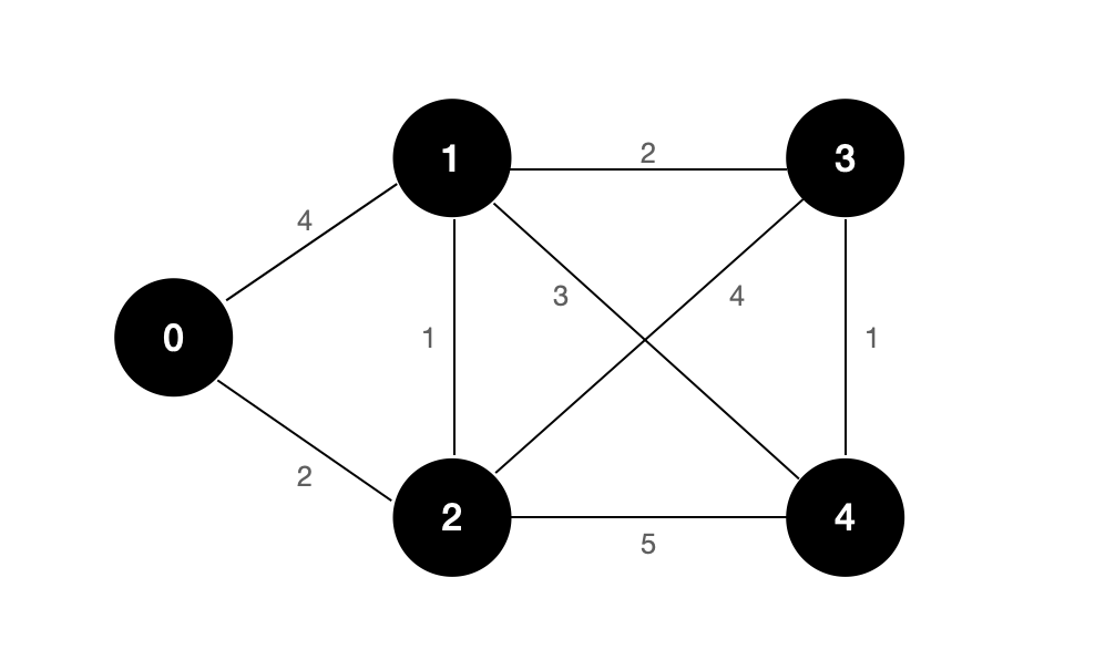
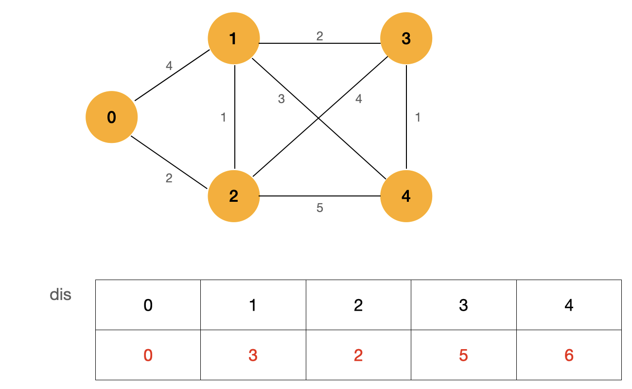
For example, the figure above shows an undirected weighted graph, and the shortest path from node 0 to node 3 is:

0 -> 2 -> 1 -> 3

Its path length is: 5.

What is the significance of studying the shortest path algorithm? Or what problems can the shortest path algorithm solve?

We know that in life, the subway is one of our important travel tools. When we input the departure and destination in the subway ticket office or software, the mobile phone software will give us the best travel scheme with the least cost or the shortest time. The realization of the function of navigation software is actually a specific application of the shortest path algorithm.

The research on the shortest path algorithm aims to solve the problems of travel, tourism and engineering cost. It is of great significance in computer science, operations research and geographic information science.

Dijkstra algorithm

Dijkstra algorithm is one of the classical algorithms for solving the shortest path of a single source. It was invented by Dijkstra, a Dutch computer scientist, in 1956.

The premise of using Dijkstra algorithm is that there can be no negative weight edges in the graph. After I introduce the idea of Dijkstra algorithm, I believe you can understand why it is the precondition of Dijkstra algorithm that the graph cannot contain negative weight edges. However, this precondition will not affect most of the problems we solve. For example, take the subway line with the lowest cost above as an example. If the weight of each edge in the graph represents the amount spent from one node to another, then the amount must be greater than 0. Therefore, Dijkstra algorithm can still solve most problems in the research field of shortest path, even if it can not deal with graphs with negative weight edges.

Next, let's look at the specific idea of Dijkstra algorithm:

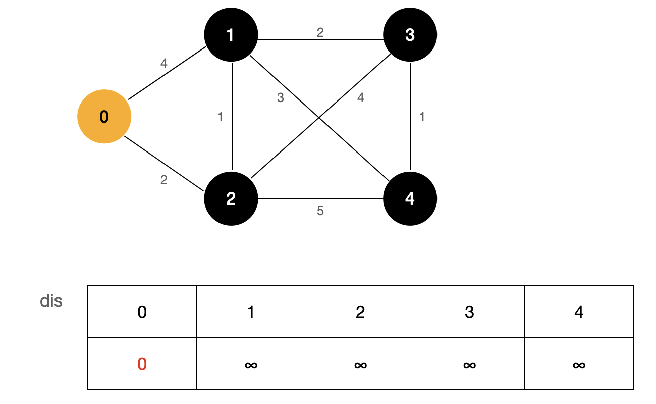
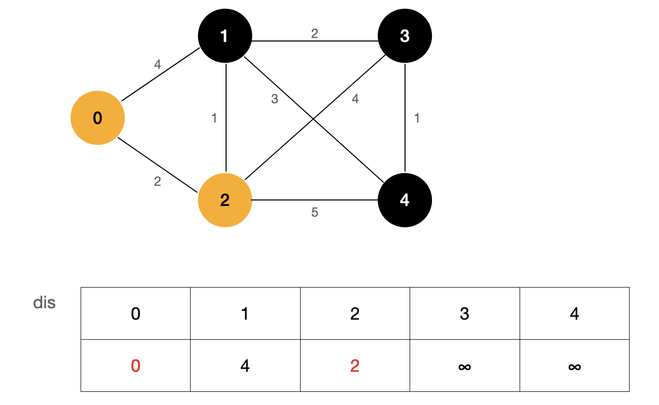
In the above figure, the source point is 0, and the table dis represents the shortest path from the source point to each point. At first, we don't know the shortest path from the source point to each point, so we use the initial value ∞ ∞ ∞, and the shortest path from the source point to the source point has been determined, and its value is 0.

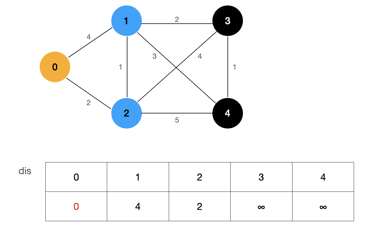
Starting from the source point, we find the nodes (1, 2) adjacent to the source point. The weight of edge 0-1 is 4 and the weight of edge 0-2 is 2. Because their value is smaller than the value in the current dis array, we update the dis array, update dis[1] to 4 and dis [2] to 2, and the weight of the remaining nodes remains ∞ ∞ ∞ . At this point, we can determine that the shortest path from the source to this point is the smallest value among these undetermined shortest path nodes.

This may be a bit of a detour. Let's take a visual look at the process through the diagram:

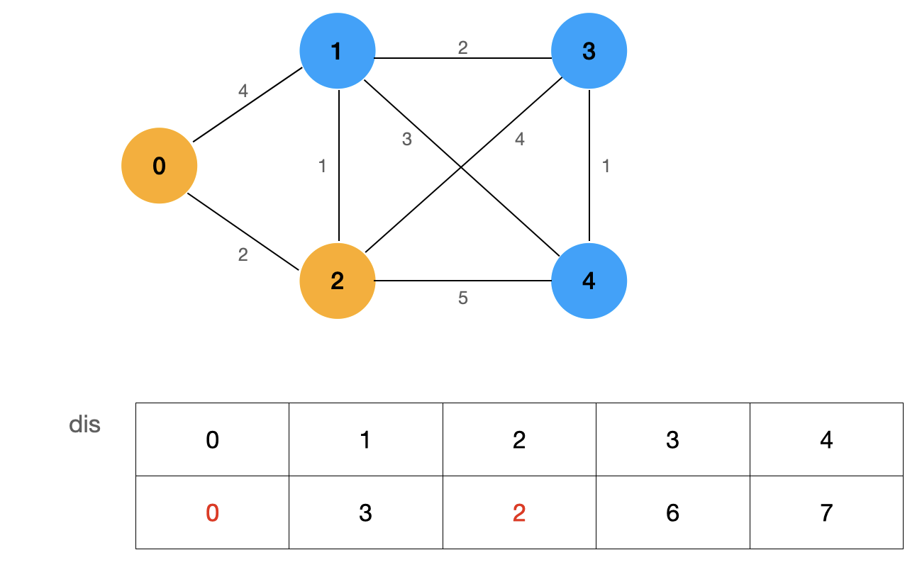
First, find the node that has determined the shortest path. In the figure, it is node 0 marked in yellow. Then update all nodes that are not determined to be the shortest path, and the blue node represents the node I updated.

Finally, among these nodes with undetermined shortest path, the shortest path is the shortest path from the source point to that point.

As shown in the figure above, the value of dis[2] is the smallest, so we can determine that the shortest path from source point 0 to node 2 is dis[2].

How can this argument be proved?

The essence of Dijkstra algorithm is greedy, which requires strict mathematical induction. I won't use mathematical derivation to prove it here. Interested friends can search [Dijkstra's algorithm: proof of correction].

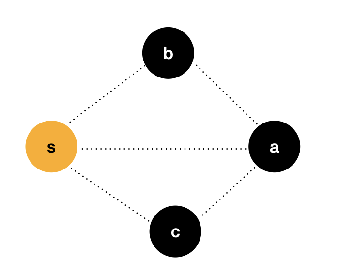
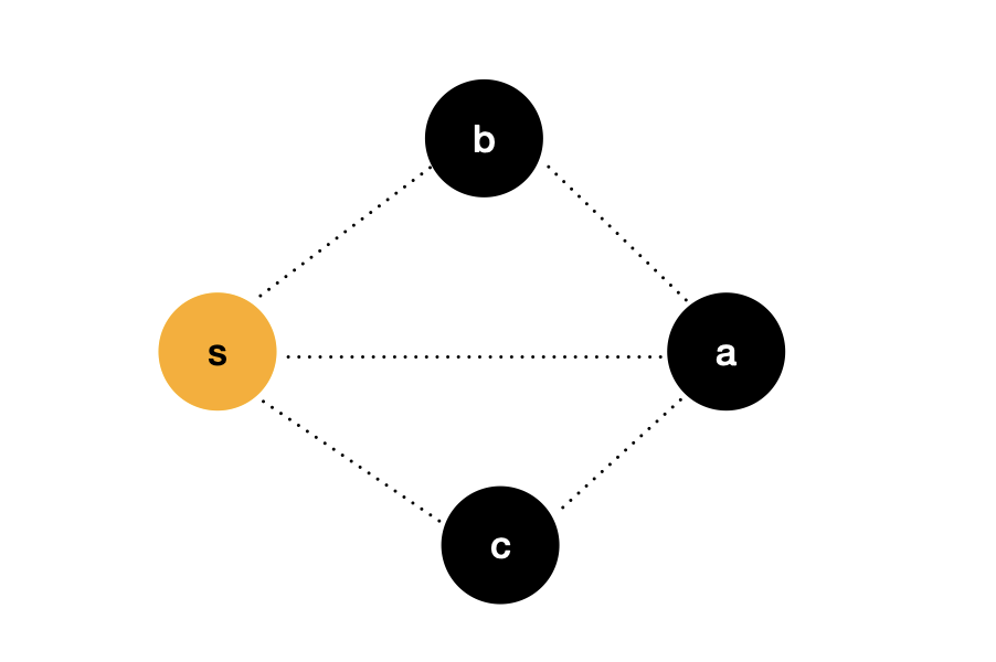
We use a more understandable way to prove the idea. In the figure above, the source point s s s to node a a a the weight of this side is recorded as d i s [ a ] dis[a] dis[a], similarly, the source point s s s to node b b b and c c c the weight of these two sides is recorded as d i s [ b ] dis[b] dis[b] and d i s [ c ] dis[c] dis[c].

Known, d i s [ a ] > d i s [ b ] dis[a] > dis[b] dis[a]>dis[b]， d i s [ a ] > d i s [ c ] dis[a] > dis[c] Dis [a] > dis [C], if there is no negative weight edge in the graph, I can be sure, d i s [ a ] dis[a] dis[a] is the source point s s s to node a a The shortest path of a.

Therefore, we can determine that the idea of Dijkstra algorithm is correct, and we also indirectly prove why the precondition of Dijkstra algorithm is that the graph cannot contain negative weight edges.

Next, we will continue to follow this idea and continue to simulate the process:

First, we update the dis array with the node that has identified the shortest path. Here, we can see that dis[1] is updated to 3. This step is also called Relaxation. The term Relaxation can be understood as that we choose to use a longer "distance" as the shortest path between two nodes. We can see that the shortest path between node 0 and node 1 is not the edge between two nodes, It's the 0-2-1 path.

We determine the node with the smallest value from the currently undetermined shortest path nodes:

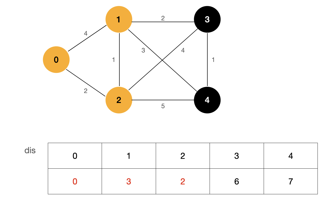
By repeating the above process, we can get the shortest path from source point 0 to all nodes in the graph:

Code implementation of Dijkstra algorithm

The Java code of Dijkstra algorithm is as follows. Because I have indicated detailed comments in the code, I will not explain the program one by one. In addition, due to the limited space of this article, I will give the link of test code at the end of the article, and the content of test cases and code will not be repeated here.

Dijkstra

import java.util.Arrays;

public class Dijkstra {

    private WeightedGraph G;
    private int s;
    private int[] dis;
    private boolean[] visited;

    public Dijkstra(WeightedGraph G, int s) {
        this.G = G;
        // Judge the legitimacy of the source point s
        if (s < 0 || s >= G.V())
            throw new IllegalArgumentException("vertex" + s + "is invalid");
        this.s = s;
        // Initialize dis array
        dis = new int[G.V()];
        Arrays.fill(dis, Integer.MAX_VALUE);
        dis[s] = 0;

        visited = new boolean[G.V()];

        // Dijkstra algorithm flow
        // 1. Find the shortest path node that is not currently accessed
        // 2. Confirm that the shortest path of this node is the current size
        // 3. According to the shortest path size of this node, find the adjacent nodes of this node and update the path length of other nodes
        while (true) {
            int curdis = Integer.MAX_VALUE;
            int cur = -1;
            
            // 1. Find the smallest node not accessed
            for (int v = 0; v < G.V(); v++)
                if (!visited[v] && dis[v] < curdis) {
                    curdis = dis[v];
                    cur = v;
                }
            
            // If cur == -1 indicates the end of all processes, jump out of the loop
            if (cur == -1) break;
            // 2. Confirm that the shortest path of this node is the current size, and update visited
            visited[cur] = true;
            // 3. According to the shortest path size of this node, find the adjacent nodes of this node and update the path length of other nodes
            for (int w : G.adj(cur))
                if (!visited[w] && dis[cur] + G.getWeight(cur, w) < dis[w])
                    dis[w] = dis[cur] + G.getWeight(cur, w);
        }
    }


    public boolean isConnected(int v) {
        if (v < 0 || v >= G.V())
            throw new IllegalArgumentException("vertex" + s + "is invalid");

        return visited[v];
    }

    public int dis(int v) {
        if (v < 0 || v >= G.V())
            throw new IllegalArgumentException("vertex" + s + "is invalid");
        return dis[v];
    }
}

We analyze the time complexity of the algorithm. The outer layer of the algorithm is a while loop, and the inner layer traverses every vertex in the graph. The termination condition of the while loop is that the shortest path of each node is determined, so the time complexity of the algorithm is O ( V 2 ) O(V^2) O(V2), where V V V is the number of vertices of the graph.

Let's think about it. Does such a Dijkstra algorithm have room for optimization? In fact, it is not difficult to find that in our algorithm class, we find the smallest node not accessed in the graph. This operation needs to traverse all nodes of the graph every time. This step can be optimized. Usually, in greedy problems, the optimization strategy is to use priority queue.

Priority queue and Pair class

Priority Queue is a special queue. In the Priority Queue, each element has its own priority, and the element with the highest priority gets the service first; Elements with the same priority are served according to their order in the Priority Queue. The Priority Queue is often implemented using the data structure of heap.

In the Java language, the default implementation of the priority queue is the minimum heap. We can use a custom comparator to specify the priority of each element of the priority queue.

In our Dijkstra algorithm class, the elements in the priority queue should maintain cur and curdis, and the priority queue should be sorted in the order of curdis from small to large.

We naturally think of customizing a class that maintains two variables cur and curdis; Then we let the class implement the Comparable interface and define our comparison logic in the compareTo method.

Here, I recommend you to use the Pair class under the com.sun.tools.javac.util package included in the JDK.

Pair

public class Pair<A, B> {
    public final A fst;
    public final B snd;

    public Pair(A var1, B var2) {
        this.fst = var1;
        this.snd = var2;
    }

    public String toString() {
        return "Pair[" + this.fst + "," + this.snd + "]";
    }

    public boolean equals(Object var1) {
        return var1 instanceof Pair && Objects.equals(this.fst, ((Pair)var1).fst) && Objects.equals(this.snd, ((Pair)var1).snd);
    }

    public int hashCode() {
        if (this.fst == null) {
            return this.snd == null ? 0 : this.snd.hashCode() + 1;
        } else {
            return this.snd == null ? this.fst.hashCode() + 2 : this.fst.hashCode() * 17 + this.snd.hashCode();
        }
    }

    public static <A, B> Pair<A, B> of(A var0, B var1) {
        return new Pair(var0, var1);
    }
}

We use Pair.fst to store cur information and Pair.snd to store curdis information. The simplified Dijkstra algorithm class using priority queue is as follows:

Dijkstra_2

import java.util.Arrays;
import java.util.Comparator;
import java.util.PriorityQueue;

public class Dijkstra_2 {
    private WeightedGraph G;
    private int s;
    private int[] dis;
    private boolean[] visited;

    public Dijkstra_2(WeightedGraph G, int s) {
        this.G = G;
        // Judge the legitimacy of the source point s
        if (s < 0 || s >= G.V())
            throw new IllegalArgumentException("vertex" + s + "is invalid");
        this.s = s;
        // Initialize dis array
        dis = new int[G.V()];
        Arrays.fill(dis, Integer.MAX_VALUE);
        dis[s] = 0;

        visited = new boolean[G.V()];

        // Dijkstra algorithm flow
        // 1. Find the shortest path node that is not currently accessed
        // 2. Confirm that the shortest path of this node is the current size
        // 3. According to the shortest path size of this node, find the adjacent nodes of this node and update the path length of other nodes

        PriorityQueue<Pair<Integer, Integer>> pq = new PriorityQueue<>(Comparator.comparingInt(o -> o.snd));
        pq.offer(new Pair<>(s, 0));

        while (!pq.isEmpty()) {
            int cur = pq.poll().fst;
            if (visited[cur]) continue;
            visited[cur] = true;
            for (int w : G.adj(cur))
                if (!visited[w] && dis[cur] + G.getWeight(cur, w) < dis[w]) {
                    dis[w] = dis[cur] + G.getWeight(cur, w);
                    pq.offer(new Pair<>(w, dis[w]));
                }
        }
    }


    public boolean isConnected(int v) {
        if (v < 0 || v >= G.V())
            throw new IllegalArgumentException("vertex" + s + "is invalid");

        return visited[v];
    }

    public int dis(int v) {
        if (v < 0 || v >= G.V())
            throw new IllegalArgumentException("vertex" + s + "is invalid");
        return dis[v];
    }
}

What is the complexity of the optimized Dijkstra algorithm?

The upper bound of the number of elements inserted in the priority queue is the number of edges in the graph E E E. The complexity of outgoing and incoming operations to the priority queue is l o g ( E ) log(E) log(E), so the time complexity of our optimized Dijkstra algorithm is O ( E l o g E ) O(ElogE) O(ElogE).

Well, that's all for the introduction of Dijkstra algorithm. We can see that the process of Dijkstra algorithm is not difficult to understand. Its idea is a greedy strategy, but our code is a little complex. If children's shoes think the code is difficult to understand, they can first try to write their own code according to their ideas, and then they can better understand the specific meaning of each sentence of the example code

Bellman Ford algorithm

In the previous chapter, we introduced Dijkstra algorithm, which mainly deals with the single source shortest path problem without negative weight edge.

So how to solve the shortest path problem for graphs with negative weight edges?

Negative weight ring

Let's take a look at this diagram:

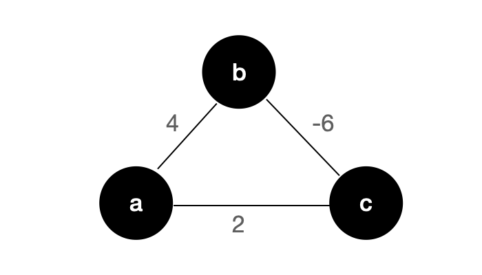
The graph is an undirected weighted graph, which requests the shortest path from node a to node c.

You might say that a - > b - > c is the shortest path from node a to node c, and its value is - 2 Wait, that doesn't seem to be the case.

For the above undirected graph, if there is a negative weight edge, there seems to be no shortest path! Because I can start from node A and go infinitely around this ring, so I can never get the shortest circuit - in fact, there is no need to turn around and waste time. After we reach node b, we can repeatedly "brush steps" on the side of b-c: -).

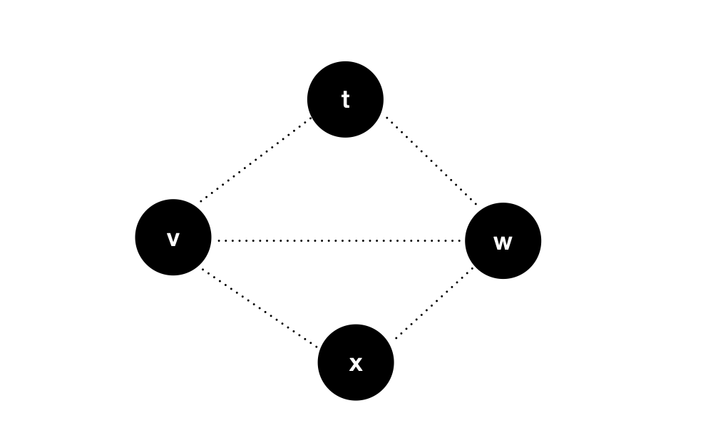
Therefore, for an undirected graph, when there is a negative weight edge, there must be no shortest path. The reason is that the negative weight edge will form a negative weight ring, and the negative weight edge of an undirected graph itself is a negative weight ring. For a directed graph, if there is a negative weight ring, there is no shortest path, such as the following figure:

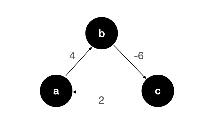
The graph is a directed graph, but there is a negative weight ring, and we can't find the shortest path.

To make a digression, the author wrote here and thought of a little story ~

The kings of countries A and B quarreled. King A was angry and stipulated that 100 yuan of country B could only be exchanged for 90 yuan of country A; After hearing this, King B also stipulated that 100 yuan in country A can only be exchanged for 90 yuan in country B. In country A, there is A smart guy who made A fortune by using this rule. Do you know how he did it? (why do you feel so retarded after writing)

Come back with the gossip.

For a graph with negative weight edges, we need to detect whether there is a negative weight ring in the graph. If there is a negative weight ring, there must be no shortest path in the graph. The detection of negative weight rings is very simple in the implementation of the algorithm. Let's take a look at a classical algorithm for solving the shortest path when there are negative weight edges - Bellman Ford algorithm.

Bellman Ford algorithm

The principle of Bellman Ford algorithm is relaxation operation.

Suppose, d i s [ v ] dis[v] dis[v] is from the source point s s s to node v v v no more than k k The shortest distance of k.

If d i s [ a ] + a b < d i s [ b ] dis[a] + ab < dis[b] Dis [a] + AB < dis [b], we will perform a relaxation operation to update d i s [ b ] = d i s [ a ] + a b dis[b] = dis[a] + ab dis[b]=dis[a]+ab；

So we found the source point s s s to node b b b no more than k + 1 k+1 The shortest distance of k+1.

Similarly, if d i s [ b ] + b a < d i s [ a ] dis[b] + ba < dis[a] Dis [b] + ba < dis [a], we perform a relaxation operation to update d i s [ a ] = d i s [ b ] + b a dis[a] = dis[b] + ba dis[a]=dis[b]+ba；

In this way, we found the source point s s s to node a a a no more than k + 1 k+1 The shortest distance of k+1.

According to the above theory, the flow of our Bellman Ford algorithm is as follows:

1. Initialize dis array, dis[s] = 0, and set other values to ∞ ∞ ∞
2. A relaxation operation is performed on all edges, and the shortest path to all points with a maximum number of edges of 1 is obtained
3. Perform another relaxation operation on all edges, and the shortest path to all points with a maximum number of edges of 2 is obtained
4. ... ...
5. After V-1 relaxation operation on all edges, the shortest path to all points with the maximum number of edges of V-1 is obtained

Our graph has only V vertices. If there is no negative weight ring, there are at most V-1 edges from one vertex to another. Therefore, after we relax all edges V-1 times, we find the shortest path from the source point to all points, and Bellman Ford algorithm supports the existence of negative weight edges.

Next, let's use an example to simulate the execution process of Bellman Ford algorithm. I believe that through this simulation process, you will have a deeper understanding of Bellman Ford algorithm: -)

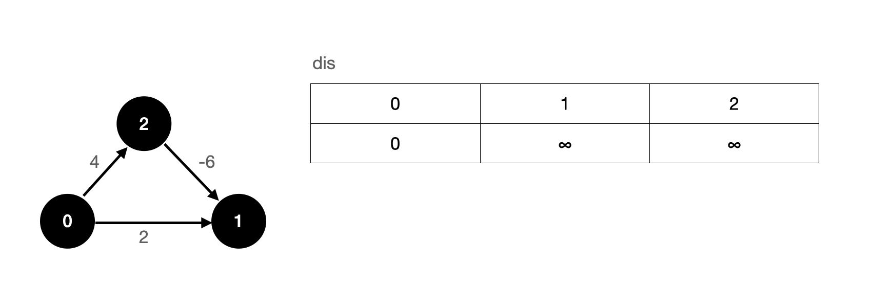
The above figure is a directed weighted graph. We specify that node 0 is the source point, the initial value of the shortest path from the source point to the source point is 0, and other nodes use it ∞ ∞ ∞.

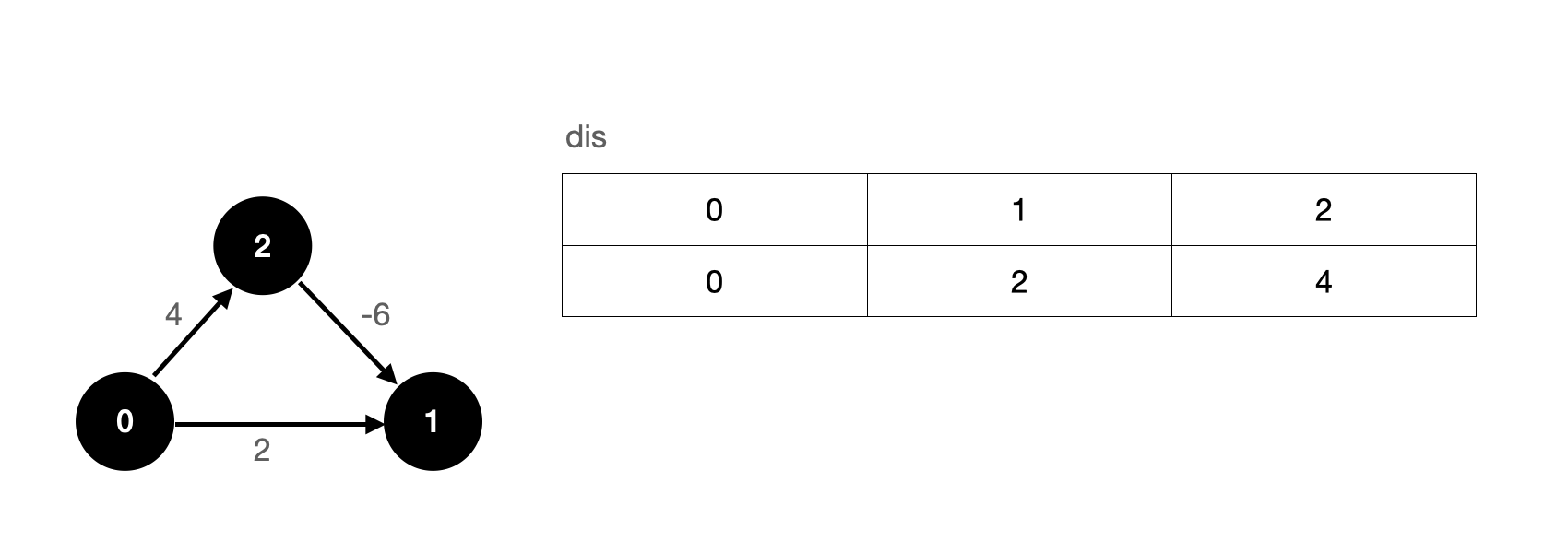
First, we perform a relaxation operation on all edges. Suppose we relax the 0-1 edge first, then the 0-2 edge, and finally the 2-1 edge. After the first relaxation operation, our dis array is updated as follows:

After the first relaxation operation, we have actually found the shortest path from the source point to each vertex.

It seems that we don't need V-1 relaxation operation? Is that so? In fact, the V-1 relaxation operation is an upper bound. It is entirely possible for us to get the result after less than V-1 relaxation operation, but in the worst case, we only need V-1 relaxation operation.

In the above example, we start from the 0-1 edge. If we change our thinking, what will be the result of starting from the 2-1 edge?

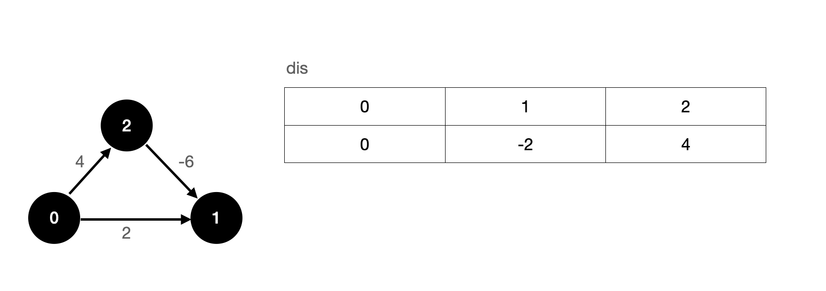
Suppose we relax the 2-1 edge first, then the 0-1 edge, and finally the 0-2 edge. After the first relaxation operation, our dis array is updated as follows:

It should be noted that when relaxing the 2-1 edge, we will use ∞ − 6 ∞ - 6 ∞− 6, which is still ∞ ∞ ∞.

After the second relaxation operation, our dis array is updated as follows:

We see that after twice relaxing all edges, we also get the correct solution.

So how to detect the negative weight ring?

In fact, it is very simple. According to Bellman Ford algorithm, if there is no negative weight ring in our graph, after V-1 relaxation operation, we can get the shortest path from the source point to each node. If we relax all edges after V-1 relaxation operation, the dis value of each point will not change; If there is a negative weight ring in the graph, after the V-1 round of relaxation operation, the relaxation operation is carried out, and each value of dis array will still change.

Therefore, in the design of the algorithm, we only need to perform another relaxation operation after V-1 relaxation operation to judge whether the dis array has changed. If it has changed, it indicates that there is a negative weight ring in the graph, that is, the shortest path cannot be obtained.

Next, let's take a look at the specific implementation of Bellman Ford algorithm.

Code implementation of Bellman Ford algorithm

The Java code of Bellman Ford algorithm is as follows. Detailed comments are indicated in the code, so I won't explain it: -)

Similarly, the link of the test code will be given at the end of the article, and the test part will not be repeated in this article.

Bellman-Ford

import java.util.Arrays;

public class BellmanFord {
    private WeightedGraph G;
    private int s;
    private int[] dis;
    public boolean hasNegativeCycle = false;

    public BellmanFord(WeightedGraph G, int s) {
        this.G = G;
        if (s < 0 || s >= G.V())
            throw new IllegalArgumentException("vertex" + s + "is invalid");
        this.s = s;
        dis = new int[G.V()];
        Arrays.fill(dis, Integer.MAX_VALUE);
        dis[s] = 0;
        // V-1 wheel slack operation
        for (int pass = 1; pass < G.V(); pass++) {

            for (int v = 0; v < G.V(); v++)
                for (int w : G.adj(v))
                    if (dis[v] != Integer.MAX_VALUE && dis[v] + G.getWeight(v, w) < dis[w])
                        dis[w] = dis[v] + G.getWeight(v, w);
        }

        // Conduct another relaxation (relaxation) operation to judge the negative weight ring
        for (int v = 0; v < G.V(); v++)
            for (int w : G.adj(v))
                if (dis[v] != Integer.MAX_VALUE && dis[v] + G.getWeight(v, w) < dis[w])
                    hasNegativeCycle = true;

    }

    public boolean isConnected(int v) {
        if (v < 0 || v >= G.V())
            throw new IllegalArgumentException("vertex" + v + "is invalid");
        return dis[v] != Integer.MAX_VALUE;
    }

    public int dis(int v) {
        if (v < 0 || v >= G.V())
            throw new IllegalArgumentException("vertex" + v + "is invalid");
        if (hasNegativeCycle) throw new RuntimeException("Exist negative cycle");
        return dis[v];
    }

}

What is the time complexity of Bellman Ford algorithm? We need to carry out V-1 round relaxation operation, and each relaxation operation will traverse all edges in the graph. Therefore, the time complexity of Bellman Ford algorithm is O ( V E ) O(VE) O(VE). It can be seen that although Bellman Ford algorithm can solve negative weight edges, its overall complexity is worse than Dijkstra algorithm.

Bellman Ford algorithm is introduced here. Next, let's take a look at the last algorithm introduced in this article - Floyd warhall algorithm.

Floyd warhall algorithm

We introduced Dijkstra and Bellman Ford to solve the shortest path of single source, and the Floyd warhall algorithm introduced in this chapter is an algorithm used to solve the shortest path of all point pairs (any two points).

What is the significance of solving all points for the shortest path?

If we know the shortest path of any two points in the graph, we can get the maximum value of the shortest path of any two points in the graph. This term is called the diameter of the graph.

For example, if our graph represents an Internet network system, and the edge between nodes represents the transmission delay of two intermediate stations, how to evaluate the performance of the network system? At this time, solving the diameter of the graph is of great significance. Solving the diameter of the graph requires solving the shortest path of all point pairs.

For Dijkstra algorithm, the complexity of solving the single source shortest path is O ( E l o g E ) O(ElogE) O(ElogE), if the shortest path of all point pairs is solved, the single source path problem needs to be solved once for each vertex in the graph. Therefore, its complexity is O ( V E l o g E ) O(VElogE) O(VElogE)； The bellman Ford algorithm is used to analyze and solve the shortest path of all point pairs, and its time complexity is O ( V 2 E ) O(V^2E) O(V2E).

For Floyd warhall algorithm, the time complexity of solving the shortest path of all points is O ( V 3 ) O(V^3) O(V3) and can solve negative weight edges. Next, let's take a look at the specific idea of Floyd warhall algorithm.

Because there is no concept of source node in Floyd warhall algorithm, or it can be considered that each node is a source node, we use one d i s dis dis array, d i s [ v ] [ w ] dis[v][w] dis[v][w] represents a vertex v v v to vertex w w The shortest path of w.

d i s dis The initialization of dis array is also very simple, d i s [ v ] [ v ] dis[v][v] The initial value of dis[v][v] is set to 0 if d i s [ v ] [ w ] dis[v][w] If dis[v][w] has an edge, then d i s [ v ] [ w ] dis[v][w] The initial value of dis[v][w] is node v v v and node w w w is the weight of this edge v w vw vw, the rest are in ∞ ∞ ∞.

The pseudo code of Floyd warhall algorithm is as follows:

for(int t = 0; t < V; t++)
  for(int v = 0; v < V; v++)
    for(int w = 0; w < V; w++)
      if(dis[v][t] + dis[t][w] < dis[v][w])
        dis[v][w] = dis[v][t] + dis[t][w]

What process does this pseudo code describe?

If node v v v and node w w There is a node between w t t t. And d i s [ v ] [ t ] + d i s [ t ] [ w ] < d i s [ v ] [ w ] dis[v][t] + dis[t][w] < dis[v][w] Dis [v] [t] + dis [t] [w] < dis [v] [w], then update d i s [ v ] [ w ] of value Value of dis[v][w] The value of dis[v][w], the essence of this step is actually a relaxation operation. So how do we understand t t What does t mean?

t t t the meaning of this cycle is that each cycle solves the intermediate process [ 0... t ] [0...t] [0...t] the shortest path of these points.

• When assigning initial values, we only consider vertices v v v and vertex w w w distance without passing any vertex;
• When t = 0 t = 0 When t=0, what we consider is if the vertex v v v and vertex w w Whether the current shortest path is updated after passing the vertex 0 in the middle of w;
• When t = 1 t = 1 When t=1, what we consider is if the vertex v v v and vertex w w w passed in the middle [ 0 , 1 ] [0,1] Whether the current shortest path is updated after the vertex in [0,1];
• When t = V − 1 t = V-1 When t=V − 1, what we consider is if the vertex v v v and vertex w w w passed in the middle [ 0... V − 1 ] [0...V-1] Whether the current shortest path is updated after the vertex in [0...V − 1].

The principle of detecting negative weight rings by Floyd warhall algorithm is actually the same as that by Bellman Ford algorithm. After the algorithm is completed, we only need to traverse all vertices of the graph d i s [ v ] [ v ] dis[v][v] Whether dis[v][v] is less than 0 is sufficient. If a negative value occurs, it indicates that the figure contains a negative weight ring.

Well, the flow of Floyd warhall algorithm is like this. Let's take a look at the specific code implementation.

Code implementation of Floyd warhall algorithm

Floyd-Warshall

import java.util.Arrays;

public class FloydWarshall {
    private WeightedGraph G;
    private int[][] dis;
    public boolean hasNegativeCycle = false;

    public FloydWarshall(WeightedGraph G) {
        this.G = G;
        dis = new int[G.V()][G.V()];
        for (int i = 0; i < G.V(); i++)
            Arrays.fill(dis[i], Integer.MAX_VALUE);

        for (int v = 0; v < G.V(); v++) {
            dis[v][v] = 0;
            for (int w : G.adj(v))
                dis[v][w] = G.getWeight(v, w);
        }

        for (int t = 0; t < G.V(); t++)
            for (int v = 0; v < G.V(); v++)
                for (int w = 0; w < G.V(); w++)
                    if (dis[v][t] != Integer.MAX_VALUE
                            && dis[t][w] != Integer.MAX_VALUE
                            && dis[v][t] + dis[t][w] < dis[v][w])
                        dis[v][w] = dis[v][t] + dis[t][w];

        for (int v = 0; v < G.V(); v++)
            if (dis[v][v] < 0) hasNegativeCycle = true;
    }

    public boolean isConnected(int v, int w) {
        if (v < 0 || v >= G.V())
            throw new IllegalArgumentException("vertex" + v + "is invalid");
        if (w < 0 || w >= G.V())
            throw new IllegalArgumentException("vertex" + w + "is invalid");
        return dis[v][w] != Integer.MAX_VALUE;
    }

    public int dis(int v, int w) {
        if (v < 0 || v >= G.V())
            throw new IllegalArgumentException("vertex" + v + "is invalid");
        if (w < 0 || w >= G.V())
            throw new IllegalArgumentException("vertex" + w + "is invalid");
        return dis[v][w];
    }
}

It can be seen that Floyd warhall algorithm is an easy to read algorithm. We can quickly see that the complexity of Floyd warhall algorithm is O ( V 3 ) O(V^3) O(V3), although this complexity is not better than Dijkstra algorithm, Floyd warhall algorithm can detect negative weight rings for graphs with negative weight edges, and its complexity is better than Bellman Ford algorithm to solve the shortest path of all point pairs.

However, the greatest advantage of Floyd warhall algorithm is its simplicity and beauty, which integrates the art of DP algorithm.

summary

In this article, I introduce you to three shortest path algorithms: Dijkstra algorithm, Bellman Ford algorithm and Floyd warhall algorithm.

Dijkstra algorithm is a classical algorithm for solving the single source shortest path. Although it can not solve the graph with negative weight edge, Dijkstra algorithm is still a very meaningful algorithm. After all, a large part of the shortest path problems we solve are without negative weight edge.

If we encounter the shortest path problem with negative weight edges, we can choose Bellman Ford algorithm or Floyd warhall algorithm. The former is used to solve the single source shortest path problem, and the latter can solve all point to shortest path problems.

Well, so far, this article has been here. Welcome to my official account. Here, I hope you can gain more knowledge, and we will see you next time!