Catalog
2. Read in data and get output
6. Model training, prediction labels
1. Preface
This article is written in the beginning of the author's in-depth learning, but the understanding is still shallow, just share what he sees and learns on the forums, ask for advice on what is wrong, and communicate friendly.
2. References and Basis
Reference Material: Deep learning by hands
Basic: have a certain understanding of the framework of in-depth learning, understand the basic operations of nd, automatic derivation
3. Why Linear Regression
As an important branch of machine learning, in-depth learning, more and more abstract concepts or patterns are represented step by step based on neural network models. Not very friendly to beginners, so we start with linear regression and softmax regression to introduce the basic concepts of in-depth learning and the basic structure of the neural network.
First, two basic single-layer neural networks, linear regression and softmax regression, are introduced.
The output predictions of a neural network are usually divided into two categories based on whether they are discrete or not, and regression is a problem if the output values are continuous. For example, forecast the price of a building, air humidity, surface temperature, and so on.
Conversely, problems that output discrete values are referred to as classification problems, such as cancer benign and malignant judgment, spam recognition, image classification.
Here, we first introduce the basic elements and representation of the in-depth learning model using linear regression as an example.
4. Problem Analysis
The most common example is a problem with home price forecasts. Until then, the price of a house depends on a number of factors, such as housing conditions, transportation, regional security, area, and so on. Here, simplifying to two factors, area and transportation, we can write the following mathematical model.
1. Modeling
The area of the house to be built is x1, traffic is x2, and the predicted output house price is , we can build an expression to predict house prices based on x1 and x2, which is the model.
Where w1 and w2 refer to weights, B is bias, they are scalars, and they are parameters of linear regression models.
Here's how model parameters are generated.
from mxnet import nd, autograd
from time import time
import random
from IPython import display
from matplotlib import pyplot as plt

# Generate Dataset
num_input = 2  # Feature Dimension
num_examples = 10000  # Number of samples
true_w = [2, -3.5]
true_b = 3.7
features = nd.random.normal(0, 1, (num_examples, num_input))
labels = true_w[0] * features[:, 0] + true_w[1] * features[:, 1] + true_b
labels += nd.random.normal(0, 0.01, shape=labels.shape)


# View data
After the model has been established. We need to read in the data to train the model and calculate each error. To reduce the error, we need to introduce an optimization algorithm to optimize the model parameters through iteration. In fact, there are already several parts left here: read in data, loss function definition, optimization algorithm writing, model training, model prediction.
2. Read in data and get output
In order to train a model, we usually collect a lot of related data, which is called training data set, a house is called a sample, where the actual price of the house sold is label, and two factors that affect the price of the house are called feature.
If the number of samples we collect is n and the index is i, the sample characteristics are And
And The prediction label is
 For samples with index i, the predictive expression of linear regression is as follows:

3. Loss function
When training a model, we need to measure the error between the output predicted value and the true label. There are usually four methods: 0-1 loss function, square loss function, absolute loss function, logarithmic loss function. The most common is the square loss function, which reflects the distance from the correct label. Its expression is as follows:
Add 1/2 to the expression to make the derivative coefficient one, which makes the form slightly simpler. Given a training set, the value of this function is only related to the parameters given to the model. In machine learning, this function is called the loss function.
In model training, our task is ultimately to find a set of parameters that minimize the average loss of training samples.
4. Optimization algorithm
Questions about solutions: analytical solutions & Numerical Solutions
When both the model and the loss function are simple, the above loss function minimization problem can be solved mathematically. This kind of solution is called analytic solution. However, most deep learning models do not have this condition and can only reduce the value of the loss function by infinite iteration of the optimization algorithm, which is called numerical solution.
Small-batch random gradient descent is widely used in optimization algorithms for solving numerical problems, and its principle is simple and not detailed here. There are two parameters that need to be set by ourselves during the iteration: (batch size),
 (learning rate), it should be emphasized that the batch size and learning rate are set artificially here, and non-model training is produced. So it's called a hyperparameter. Of course, in rare cases, hyperparameters can also be obtained from model training, which is not discussed in detail here.
Specific implementation:
# Reading datasets
def data_iter(batch_size, features, labels):
    num_examples = len(features)
    index = list(range(num_examples))
    random.shuffle(index)
    for i in range(0, num_examples, batch_size):
        j = nd.array(index[i: min(i + batch_size, num_examples)])
        yield features.take(j), labels.take(j)
batch_size = 10
# View data
# for x, y in data_iter(batch_size,features ,labels):
#     print('\n',n,x,y)
#     break

# Define Model
def linreg(x, w, b):
    return nd.dot(x, w) + b


# Define loss function
def square_loss(y_hat, y):
    return ( y_hat- y.reshape(y_hat.shape)) ** 2 / 2


# Define an optimization algorithm
def sgd(params, lr, batch_size):
    for param in params:
        param[:] = param - lr * param.grad / batch_size
6. Model training, prediction labels
Realization:
# Initialization parameters
w = nd.random.normal(0, 0.01, (num_input, 1))
b = nd.zeros(1,)
w.attach_grad()
b.attach_grad()
# print(w ,b)
# Start training
net = linreg
loss = square_loss
lr = 0.01
epochs = 5
for epoch in range(epochs):
for x, y in data_iter(batch_size, features, labels):
with autograd.record():
l = loss(net(x, w, b), y)
l.backward()
sgd([w, b], lr, batch_size)
train_l = loss(net(features, w, b), labels)
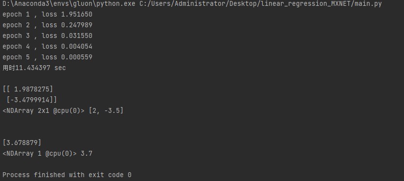
print('epoch %d , loss %f' % (epoch + 1, train_l.mean().asnumpy()))
print("Time-consuming%f sec"%(time()-stat))
print(w,true_w,'\n')
print(b,true_b)
Output results: