Objective: to predict whether a college student can be admitted to the university according to the score.

Methods: call the advanced optimization algorithm or write the gradient descent function (choose the learning rate and iteration times by yourself)

Data: ex2data1 txt

1, Read in data.

1.1 INTRODUCTION Kit

import numpy as np
import pandas as pd
import scipy.optimize as opt
import matplotlib.pyplot as plt

1.2 import data

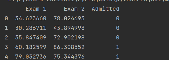
 path = '../data/exc_2/ex2data1.txt'
 data = pd.read_csv(path, header=None, names=["Exam 1", 'Exam 2', "Admitted"])
 print(data.head())

                

1.3 data visualization:

positive = data[data['Admitted'].isin([1])]
negative = data[data['Admitted'].isin([0])]

fig, ax = plt.subplots(figsize=(12, 8))
ax.scatter(positive['Exam 1'], positive['Exam 2'], s=50,c='b', marker='o', label='Admitted')
ax.scatter(negative['Exam 1'], negative['Exam 2'], s=50, c='r', marker='x', label='Not Admitted')
ax.legend()
ax.set_xlabel('Exam 1 Score')
ax.set_ylabel('Exam 2 Score')
plt.show()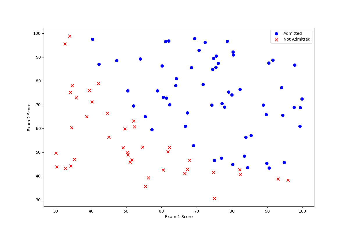

1.4} extract data x, y and initialize theta

data.insert(0, "Ones", 1)
x = np.matrix(data2.iloc[:, :-1])
y = np.matrix(data2.iloc[:, -1])
y = y.reshape(y.shape[1], 1)
theta = np.matrix(np.zeros(3))

II. Advanced optimization algorithm

If we directly call the advanced optimization function, we can easily get the minimum value without specifying the number of iterations and learning rate. Just write the calculation gradient and cost function. (Note: the gradient function written by theta is only updated)

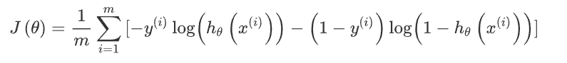
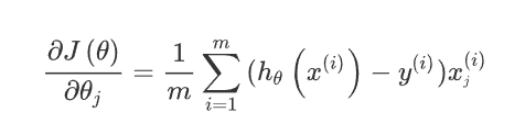
According to the formula:

Cost function:

                        

Gradient:

The reason why this is the form here is because of our h_theta (x) is the sigmoid function.

That is, g(z) = 1 / (1 + e^z)

So we need to define the following functions:

1. sigmoid

def sigmoid(z):
    return 1 / (1 + np.exp(-z))

2. Calculate gradient

def gradient2(theta, x, y):
    theta = np.matrix(theta)
    x = np.matrix(x)
    y = np.matrix(y)
    parameters = int(theta.shape[1])
    # print(parameters)
    gap = sigmoid(x * theta.T) - y
    grad = np.zeros(parameters)
    for i in range(parameters):
        term = np.multiply(gap, x[:, i])
        grad[i] = np.sum(term) / len(x)
    # term = np.multiply(gap, x)
    # print(term)
    # Print ("shape of term:", term.shape)
    return grad

 3. Cost function

def cost_tmp(theta, x, y):
    theta = np.matrix(theta)
    x = np.matrix(x)
    y = np.matrix(y)
    term = np.multiply(-y, np.log(sigmoid(x * theta.T))) - np.multiply((1 - y), np.log(1 - sigmoid(x * theta.T)))
    return np.sum(term) / len(x)

Call Fmin directly_ TNC can obtain the following results:

result = opt.fmin_tnc(func=cost_tmp, x0=theta, fprime=gradient2, args=(x, y))
print("the func cost is: ", cost_tmp(result[0], x, y))
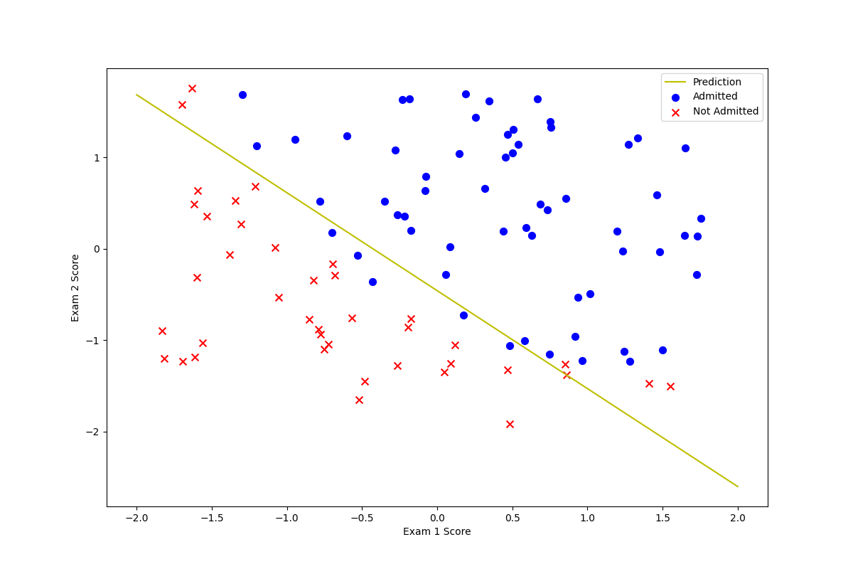
print("the func g is: ", result[0])

Visualize it:

    plotting_x1 = np.linspace(30, 100, 100)
    plotting_h1 = (- result[0][0] - result[0][1] * plotting_x1) / result[0][2]

    fig, ax = plt.subplots(figsize=(12, 8))
    ax.plot(plotting_x1, plotting_h1, 'y', label='Prediction')
    ax.scatter(positive['Exam 1'], positive['Exam 2'], s=50, c='b', marker='o', label='Admitted')
    ax.scatter(negative['Exam 1'], negative['Exam 2'], s=50, c='r', marker='x', label='Not Admitted')
    ax.legend()
    ax.set_xlabel('Exam 1 Score')
    ax.set_ylabel('Exam 2 Score')
    plt.show()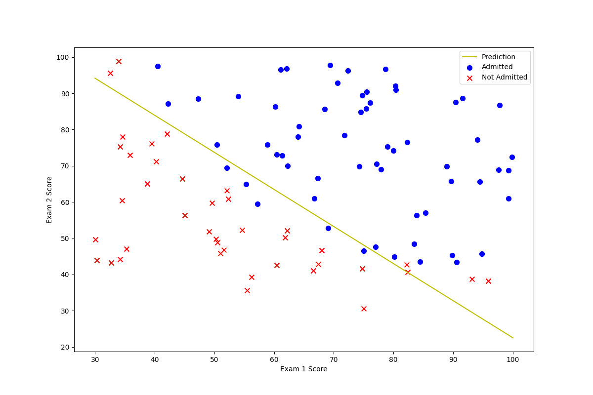

 

 

--------------------------------------- the following is the method (and problems encountered) of manually realizing gradient descent------------------------------------

The cost function and sigmoid are the same as above. The difference is that when calculating the gradient, we need to update the value of theta

According to the formula in the figure, the following code can be written.

Pay attention to the H here_ Theta (x) is different from the previous linear regression.

def TestDecend(theta, x, y, times, alpha):
    # Here is the gradient descent, then we apply the formula:
    # theta_0: should be: theta_0 = theta_0 - (alpha * ((difference * 1)) / m (m is the number of samples)
    # theta_ 1: theta_ 1 = theta_ 1 - (alpha * (difference * corresponding x_i)) / M
    numoftheta = int(theta.shape[1])
    temp = np.matrix(np.zeros(theta.shape))
    ct = np.zeros(times)

    for i in range(times):
        # Calculate the difference
        error = sigmoid(x * theta.T) - y  # Under this theta, the difference between the predicted value and the real value y.
        # Start calculating theta_ 0, theta_ one
        for j in range(numoftheta):  # Number of parameters
            # Start updating theta
            term = np.multiply(error, x[:, j])  # The above formula. Difference * 1 or difference * x_i
            temp[0, j] = theta[0, j] - (alpha * np.sum(term)) / len(x)

        theta = temp
        ct[i] = cost(theta, x, y)
        # print("the cost of this iteration is updated to:", cost[i])
    return theta, ct

If we directly, without data processing, call the gradient descent written by ourselves. Namely:

    times = 15000
    alpha = 0.08
    g, c = TestDecend(theta, x, y, times, alpha)  # The problem encountered before is that there is no way to implement the same functions as the above. The reason is that there is no normalization

    g = np.matrix.tolist(g)
    print("the testDescen g is: ", g, type(g))

    print("the cost is: ", c)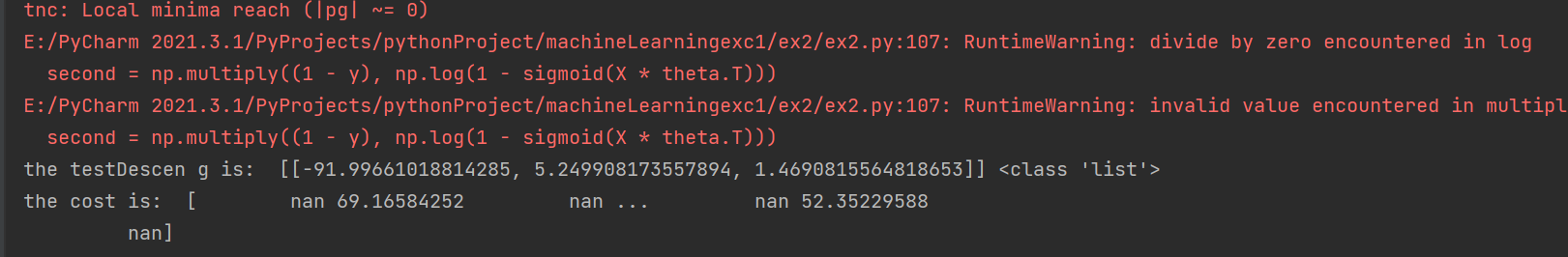

 

It will appear that in the cost calculation, the divisor is zero. And you can see that cost will have a nan value.

We observed the fitting of the final curve and data. Is completely biased (under fitted):

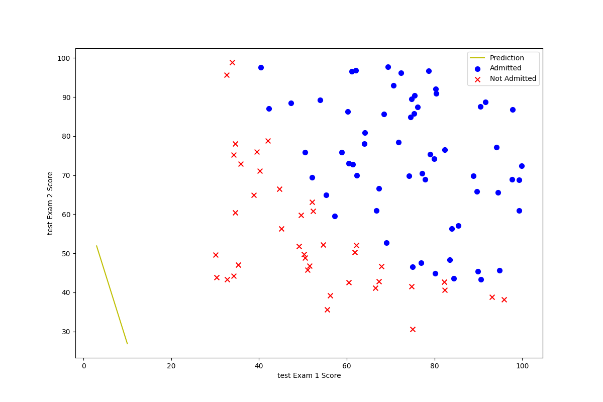
At that time, this question puzzled me for a long time. In principle, there is no problem with our gradient descent function. How could this happen?

Later, notice that when we read data, the range of exam1 and exam2 data is different. So we need to normalize it. Therefore, when reading data, we should deal with it in this way.  

#  To achieve manual gradient descent, the data must be normalized. (except for admitted, otherwise the divisor will be zero or cannot be fitted at all)
data2.iloc[:, :-1] = (data2.iloc[:, :-1] -     data2.iloc[:, :-1].mean()) / data2.iloc[:, :-1].std()
print(data2.head())

Let's call it again and compare whether the result is consistent with that of the advanced optimization function:

 

    result = opt.fmin_tnc(func=cost_tmp, x0=theta, fprime=gradient2, args=(x, y))
    print("the func cost is: ", cost_tmp(result[0], x, y))
    print("the func g is: ", result[0])

    #
    times = 15000
    alpha = 0.08
    g, c = TestDecend(theta, x, y, times, alpha)  # The problem encountered before is that there is no way to implement the same functions as the above. The reason is that there is no normalization

    g = np.matrix.tolist(g)
    print("the testDescen g is: ", g, type(g))

    print("the cost is: ", c)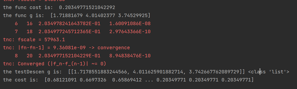

It can be found that this is roughly the same. At the same time, we visualize the data.

 

It can be seen that the fitting degree is consistent with the effect of advanced optimization algorithm.