Single layer perceptron
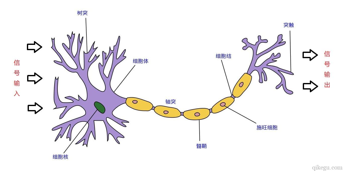
Biological neuron
The structure of nerve cells can be roughly divided into dendrites, synapses, cell bodies and axons. A single nerve cell can be regarded as a machine with only two states - yes when excited and no when not excited. The state of nerve cells depends on the amount of input signals received from other nerve cells and the strength of synapses (inhibition or enhancement). When the sum of signals exceeds a certain threshold, the cell body will be excited and produce electrical pulses. Electrical pulses are transmitted to other neurons along axons and through synapses. In order to simulate the behavior of nerve cells, the corresponding basic concepts of perceptron are proposed, such as weight (synapse), bias (threshold) and activation function (cell body).
perceptron
Inspired by biological neural network, computer scientist Frank Rosenblatt proposed an artificial neural network structure simulating biological neural network in the 1960s, which is called Perceptron. Like the above neuron cells, the Perceptron also has two states. Its essence is a binary linear classification model. The input is the feature vector of the instance, the output is the category of the instance, and the binary values of + 1 and - 1 are taken.

x 1 ... x n x_1\dots x_n x1... xn bit each component of n-dimensional input vector.
w 1 ... w n w_1\dots w_n w1... wn is the weight (weight) of each input component connected to the perceptron, which can adjust the size of the input vector value to make the input signal larger (W > 0), unchanged (w=0) or reduced (W < 0). It can be understood as the signal function in biological neural network. The signal will change when it is transmitted to the nucleus through dendrites.
w 0 w_0 w0 = offset
First step
Here, z is called net input, and its value is equal to the sum of each dimension value x of a sample multiplied by the weight value w corresponding to the dimension.
z
=
w
0
x
0
+
w
1
x
1
+
w
2
x
2
+
⋯
+
w
n
x
n
=
∑
i
=
0
n
w
i
x
i
=
W
T
X
z=w_0x_0+w_1x_1+w_2x_2+\dots+w_nx_n=\sum_{i=0}^nw_ix_i=W^TX
z=w0x0+w1x1+w2x2+⋯+wnxn=i=0∑nwixi=WTX
Step 2
Where z is called net input. However, such a calculation result is a continuous value, and the output of the perceptron is + 1 and - 1 binary. Therefore, we need to convert the result into discrete classification values. Here we use a conversion function, which is called excitation function (activation function).
s
i
g
n
(
z
)
=
{
+
1
,
z
≥
0
−
1
,
z
<
0
sign(z)=\begin{cases} +1, &z\ge0\\ -1, &z\lt0\\ \end{cases}
sign(z)={+1,−1,z≥0z<0
y = s i g n ( ∑ i = 0 n w i x i ) y=sign(\sum_{i=0}^nw_ix_i) y=sign(i=0∑nwixi)
x i x_i xi represents the j-th feature of the i-th sample
Step 3
Perceptron is a self-learning algorithm, which can continuously adjust the weight update according to the input data, and finally complete the classification. The weight update formula is as follows:
w
i
=
w
i
+
Δ
w
i
Δ
w
i
=
η
(
t
−
y
)
x
i
\begin{aligned} &w_i=w_i+Δw_i \\ &Δw_i=η(t-y)x_i \end{aligned}
wi=wi+ΔwiΔwi=η(t−y)xi
η Is the learning rate, t is the real value,
y
y
y is the predicted value
Note: the weight update basis of the perceptron is: if the prediction is accurate, the weight will not be updated; otherwise, the weight will be increased to make it more tend to the correct category.
code implementation
Simple implementation
import numpy as np
import matplotlib.pyplot as plt

#input data
X = np.array([[1, 3, 3],
              [1, 4, 3],
              [1, 1, 1],
              [1, 0, 2]])

#label
Y = np.array([[1],
             [1],
             [-1],
             [-1]])

#Weight initialization, 3 rows and 1 column, value range - 1 to 1
W = (np.random.random([3,1])-0.5)*2
print(W)

#Learning rate setting
lr = 0.11
#Neural network output
O = 0

def update():
    global X,Y,W,lr
    O = np.sign(np.dot(X,W))
    #Because the matrix is used here, the computer result of X.T*(Y-O) is the sum of rows multiplied by columns, so it needs to be divided by the number of data (or not divided)
    W_C = lr*(X.T.dot(Y-O))/X.shape[0]
    W = W + W_C

for i in range(100):
    update()#Update weight
    print(W)#Print current weight
    print(i)#Print iterations
    O = np.sign(np.dot(X,W))#Calculate current output
    if(O == Y).all():#The predicted values are all equal to the real values
        print('Finished')
        print('epoch',i)
        break
Classification of iris
import numpy as np
import pandas as pd
from sklearn.datasets import load_iris
from sklearn.model_selection import train_test_split

# Return a tuple and unpack the tuple.
X, y = load_iris(return_X_y=True)
# Merge X and y. Note that when merging, you need to convert y into a two-dimensional array.
data = pd.DataFrame(np.concatenate((X, y.reshape(len(y), -1)), axis=1))
# Duplicate records exist in iris dataset, please delete.
data.drop_duplicates(inplace=True)
len(data)
# The mapping is 1 and - 1 in order to match the value predicted by the perceptron.
data[4] = data[4].map({0:1, 1:-1, 2:2})
# Filter iris data with category 2.
data = data[data[4] != 2]
# data.shape

class Perceptron:
    """use Python Language implementation perceptron. Second classification."""

    def __init__(self, alpha, times):
        """Initialization method.

        Parameters
        -----
        alpha : float
            Learning rate.
        times : int
            Maximum number of iterations.
        """
        self.alpha = alpha
        self.times = times

    def step(self, z):
        """Step function.

        Parameters
        -----
        z : Array type (or scalar type).
            Parameters of step function. That is, the net input of the perceptron.

        Returns
        -----
        value : int
            If z >= 0,Return 1, otherwise return-1.
        """
        return np.where(z >= 0, 1, -1)

    def fit(self, X, y):
        """According to the provided training data, the model is trained.

        Parameters
        -----
        X : Class array type. Shape is[Number of samples]
            The characteristic attributes of the samples to be trained.
        y : Class array type, shape[Number of samples]
            Target value (label) for each sample.
        """
        X = np.asarray(X)
        y = np.asarray(y)
        # Create a vector of weights, with an initial value of 0 and a length of 1. (the extra value is intercept)
        self.w_ = np.zeros(1 + X.shape[1])
        # Create a loss list to save the loss value after each iteration.
        self.loss_ = []
        # Cycle the specified number of times.
        for i in range(self.times):
            # Define the loss value per cycle, that is, the number of prediction errors.
            loss = 0
            # Each sample in the training set (feature x and target tag y) is obtained in turn.
            for x, target in zip(X, y):
                # Calculate the predicted value.
                y_hat = self.step(np.dot(x, self.w_[1:]) + self.w_[0])
                # If the predicted value does not match the real value, the error will be increased.
                loss += y_hat != target
                # Calculate the updated gradient value. The calculation method is: δ w(j) = learning rate * (real target value - predicted value) * x(j)
                # w += δw
                # Update the weights.
                self.w_[0] += self.alpha * (target - y_hat)
                self.w_[1:] += self.alpha * (target - y_hat) * x
            # Add the error accumulated in the cycle to the error list.
            self.loss_.append(loss)

    def predict(self, X):
        """Predict the sample data according to the samples transmitted by the parameters.

        Parameters
        -----
        X : Class array type, shape[Number of samples, Number of features]
            Sample characteristics (attributes) to be tested

        Returns
        -----
        result : Array type.
            Predicted results (classification values).
        """
        return self.step(np.dot(X, self.w_[1:]) + self.w_[0])

X, y = data.iloc[:, 0:4], data[4]
train_X, test_X, train_y, test_y = train_test_split(X, y, test_size=0.2, random_state=0)
p = Perceptron(0.1, 10)
p.fit(train_X, train_y)
result = p.predict(test_X)
display(result)
display(test_y.values)
display(p.w_)
display(p.loss_)
display(np.sum(result == test_y) / len(result))


import matplotlib as mpl
import matplotlib.pyplot as plt
# Set the font to bold to display Chinese normally.
mpl.rcParams["font.family"] = "SimHei"
# When the Chinese font is set, the negative sign can be displayed normally.
mpl.rcParams["axes.unicode_minus"]=False


# Draw true values
plt.plot(test_y.values, "go", ms=15, label="True value")
# Draw the predicted value
plt.plot(result, "rx", ms=15, label="Estimate")
plt.title("Perceptron two classification")
plt.xlabel("Sample serial number")
plt.ylabel("category")
plt.legend()
plt.show()

# Draw objective function loss value
plt.plot(range(1, p.times + 1), p.loss_, "o-")
.values, "go", ms=15, label="True value")
# Draw the predicted value
plt.plot(result, "rx", ms=15, label="Estimate")
plt.title("Perceptron two classification")
plt.xlabel("Sample serial number")
plt.ylabel("category")
plt.legend()
plt.show()

# Draw objective function loss value
plt.plot(range(1, p.times + 1), p.loss_, "o-")