Article directory
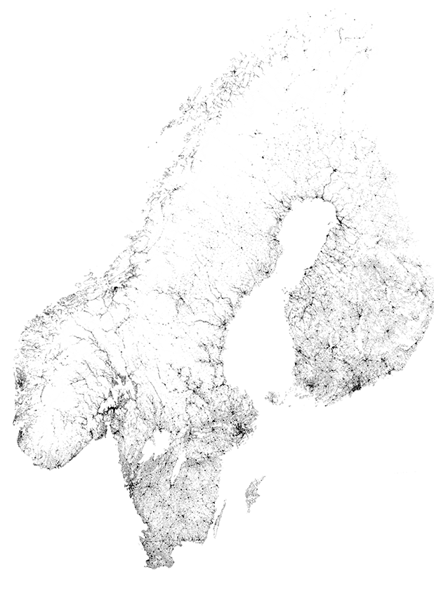
Opening picture
SIR model of infectious diseases
- S is the number of healthy people
- I is the number of people infected
- R is the number of people recovered
u(t)=(SIR) u(t) = \begin{pmatrix} S \\ I \\ R \end{pmatrix}u(t)=⎝⎛SIR⎠⎞
The dynamic model of evolution is a system of first order ordinary differential equations
f(u)=u′(t)=(S′I′R′)=(−βISβIS−γIγI)un+1=f(u)Δt+un
f(u) = u'(t) = \begin{pmatrix} S' \\ I' \\ R' \end{pmatrix} = \begin{pmatrix}
-\beta I S \\
\beta I S - \gamma I \\
\gamma I
\end{pmatrix} \\
u_{n+1} = f(u)\Delta t + u_n
f(u)=u′(t)=⎝⎛S′I′R′⎠⎞=⎝⎛−βISβIS−γIγI⎠⎞un+1=f(u)Δt+un
There are two parameters in the model: β, γ \ beta, gamma β, γ, which represent the infection rate and recovery rate respectively.
The above model describes the changes in the number of patients in a single population.
If we want to consider geospatial propagation, we need to further modify the model. It can be assumed that the geographical space is divided into grids, and infectious diseases can be transmitted through adjacent grids.
Obviously, this model is not reliable, but it can be used for visualization:
f(u)=u′(t)=(S′I′R′)=(−β(Si,jIi,j+Si−1,jIi−1,j+Si+1,jIi+1,j+Si,j−1Ii,j−1+Si,j+1Ii,j+1)β(Si,jIi,j+Si−1,jIi−1,j+Si+1,jIi+1,j+Si,j−1Ii,j−1+Si,j+1Ii,j+1)−γIi,jγIi,j) f(u) = u'(t) = \begin{pmatrix} S' \\ I' \\ R' \end{pmatrix} = \begin{pmatrix} -\beta \left(S_{i,j}I_{i,j} + S_{i-1,j}I_{i-1,j} + S_{i+1,j}I_{i+1,j} + S_{i,j-1}I_{i,j-1} + S_{i,j+1}I_{i,j+1}\right) \\ \beta \left(S_{i,j}I_{i,j} + S_{i-1,j}I_{i-1,j} + S_{i+1,j}I_{i+1,j} + S_{i,j-1}I_{i,j-1} + S_{i,j+1}I_{i,j+1}\right) - \gamma I_{i,j} \\ \gamma I_{i,j} \end{pmatrix}f(u)=u′(t)=⎝⎛S′I′R′⎠⎞=⎝⎛−β(Si,jIi,j+Si−1,jIi−1,j+Si+1,jIi+1,j+Si,j−1Ii,j−1+Si,j+1Ii,j+1)β(Si,jIi,j+Si−1,jIi−1,j+Si+1,jIi+1,j+Si,j−1Ii,j−1+Si,j+1Ii,j+1)−γIi,jγIi,j⎠⎞
Code
import numpy as np
import math
import matplotlib.pyplot as plt
%matplotlib inline
from matplotlib import rcParams
import matplotlib.image as mpimg
rcParams['font.family'] = 'serif'
rcParams['font.size'] = 16
rcParams['figure.figsize'] = 12, 8
from PIL import Image
SIR
beta = 0.010
gamma = 1

def f(u):
    S = u[0]
    I = u[1]
    R = u[2]

    new = np.array([-beta*(S[1:-1, 1:-1]*I[1:-1, 1:-1] + \
                            S[0:-2, 1:-1]*I[0:-2, 1:-1] + \
                            S[2:, 1:-1]*I[2:, 1:-1] + \
                            S[1:-1, 0:-2]*I[1:-1, 0:-2] + \
                            S[1:-1, 2:]*I[1:-1, 2:]),
                     beta*(S[1:-1, 1:-1]*I[1:-1, 1:-1] + \
                            S[0:-2, 1:-1]*I[0:-2, 1:-1] + \
                            S[2:, 1:-1]*I[2:, 1:-1] + \
                            S[1:-1, 0:-2]*I[1:-1, 0:-2] + \
                            S[1:-1, 2:]*I[1:-1, 2:]) - gamma*I[1:-1, 1:-1],
                     gamma*I[1:-1, 1:-1]
                    ])

    padding = np.zeros_like(u)
    padding[:,1:-1,1:-1] = new
    padding[0][padding[0] < 0] = 0
    padding[0][padding[0] > 255] = 255
    padding[1][padding[1] < 0] = 0
    padding[1][padding[1] > 255] = 255
    padding[2][padding[2] < 0] = 0
    padding[2][padding[2] > 255] = 255

    return padding
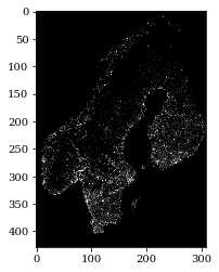
Prepare a population density map
In order to use the pixel value to represent the number of people, you need to flip black and white
from PIL import Image
img = Image.open('popdensity.png')
img = img.resize((img.size[0]//2,img.size[1]//2))
img = 255 - np.asarray(img)
plt.imshow(img)
Numerical solution of initial value problem by Euler method
The initial conditions are:
- S number of healthy people is equal to the value of population density map
- I the initial number of infections is 0, and the location of disease outbreak is set to 1
- R complex number is initially 0
S_0 = img[:,:,1]
I_0 = np.zeros_like(S_0)
I_0[309,170] = 1 # patient zero
R_0 = np.zeros_like(S_0)

T = 900                         # final time
dt = 1                          # time increment
N = int(T/dt) + 1               # number of time-steps
t = np.linspace(0.0, T, N)      # time discretization

# initialize the array containing the solution for each time-step
u = np.empty((N, 3, S_0.shape[0], S_0.shape[1]))
u[0][0] = S_0
u[0][1] = I_0
u[0][2] = R_0

def euler_step(u, f, dt):
    return u + dt * f(u)

for n in range(N-1):
    u[n+1] = euler_step(u[n], f, dt)
Custom colormap
The following code changes the transparency so that the two pictures are drawn together
import matplotlib.cm as cm
theCM = cm.get_cmap("Reds")
theCM._init()
alphas = np.abs(np.linspace(0, 1, theCM.N))
theCM._lut[:-3,-1] = alphas
Draw GIF
import matplotlib.animation as animation

n_frames =45

def draw(i):
    plt.imshow(img, vmin=0, vmax=255, interpolation="nearest")
    plt.imshow(u[i][1], vmin=0, cmap=theCM, interpolation="nearest")
    plt.xticks([])
    plt.yticks([])


height, width, depth = img.shape
dpi = 100
fig = plt.figure(figsize=(width // dpi, height // dpi))
fig.clf()
ax = fig.subplots()

fps = 3
ani = animation.FuncAnimation(fig, draw, frames=range(0, N-1, N//n_frames), interval=1000/fps, repeat=True)
ani.save('change.gif', writer='pillow', fps=fps)
# plt.show()
The results are shown at the beginning!

