1. Principal Component Analysis (PCA) Thought and Principle

1.1 What is principal component analysis

PCA(Principal Component Analysis), a principal component analysis method, is the most widely used data dimension reduction algorithm (unsupervised machine learning method).

Its main purpose is to "reduce dimensionality", by disjuncting the largest individual differences of principal components, to discover features that are more easily understood by humans. It can also be used to reduce the number of variables in regression and cluster analysis.

1.2 Why do you want to do principal component analysis?

In many scenarios, multivariable data needs to be observed, which increases the workload of data collection to some extent. More importantly, there may be a correlation between multivariates, which increases the complexity of problem analysis.

If each index is analyzed separately, the results of the analysis are often isolated and do not fully utilize the information in the data, so blindly reducing the index will lose a lot of useful information, resulting in incorrect conclusions.

Therefore, it is necessary to find a reasonable method to minimize the loss of information contained in the original indicators while reducing the indicators that need to be analyzed in order to comprehensively analyze the collected data. Because there is a certain correlation between the variables, it is possible to consider making the closely related variables as few new variables as possible, so that the new variables are not related to each other, then less comprehensive indicators can be used to represent the various information existing in each variable. Principal component analysis and factor analysis belong to this kind of dimension reduction algorithm.

1.3PCA Approximate Process

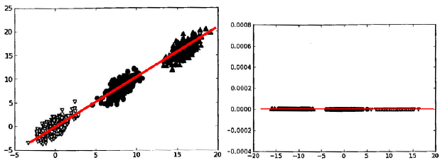
What PCA needs to do is simply find a set of orthogonal coordinate axes in the original space sequentially. The first axis makes the variance maximum, the second axis makes the variance maximum in the plane orthogonal to the first axis, and the third axis makes the variance maximum in the plane orthogonal to the first and second axes. This assumes that in N-dimensional space, We can find N such axes, and we take the first R to approximate this space so that we can compress from an N-dimensional space to an r-dimensional space, but we choose r axes to minimize the loss of data due to the compression of space.

Therefore, the key point is how to find a new projection direction to minimize the loss of "information" from the original data.

1.4 Measurement of sample information

The "amount of information" of a sample refers to the variance of the projection of the sample in the characteristic direction. The larger the variance, the greater the difference in this feature between samples, and therefore the more important this feature is. As illustrated in the illustration in Machine Learning Practice, the larger the variance of the samples, the easier it is to distinguish the samples of different classes.

2. Algorithmic implementation

2.1 Introducing Related Libraries

# Add directory to system path for easy module import. The root directory of the project is'.../machine-learning-toy-code'
import sys
from pathlib import Path
curr_path = str(Path().absolute())
parent_path = str(Path().absolute().parent)
p_parent_path = str(Path().absolute().parent.parent)
sys.path.append(p_parent_path) 
print(f"The home directory is:{p_parent_path}")
from torch.utils.data import DataLoader
from torchvision import datasets
import torchvision.transforms as transforms
import matplotlib.pyplot as plt
import numpy as np

from sklearn.decomposition import PCA
import numpy as np
import matplotlib.pyplot as plt

2.2 Dimension reduction using PCA

train_dataset = datasets.MNIST(root = p_parent_path+'/datasets/', train = True,transform = transforms.ToTensor(), download = False)
test_dataset = datasets.MNIST(root = p_parent_path+'/datasets/', train = False, 
                               transform = transforms.ToTensor(), download = False)

batch_size = len(train_dataset)
train_loader = DataLoader(dataset=train_dataset, batch_size=batch_size, shuffle=True)
test_loader = DataLoader(dataset=test_dataset, batch_size=batch_size, shuffle=True)
X_train,y_train = next(iter(train_loader))
X_test,y_test = next(iter(test_loader))
X_train,y_train = X_train.cpu().numpy(),y_train.cpu().numpy() # tensor to array)
X_test,y_test = X_test.cpu().numpy(),y_test.cpu().numpy() # tensor to array)
X_train = X_train.reshape(X_train.shape[0],784)
X_test = X_test.reshape(X_test.shape[0],784)
m , p = X_train.shape # m: number of training sets, p: number of characteristic dimensions
print(f"Original characteristic dimension number:{p}") # The number of feature dimensions is 784

# N_ When components are integers >=1, they represent the number of characteristic dimensions after the expected PCA dimensionality reduction
# N_ When components are [0,1], they represent the variance of the principal components and the minimum proportional threshold occupied by them, and the PCA class itself determines the dimension to which the reduction is based on the variance of the sample characteristics.
model = PCA(n_components=0.95) 
lower_dimensional_data = model.fit_transform(X_train)
print(f"The number of characteristic dimensions after dimension reduction:{model.n_components_}")

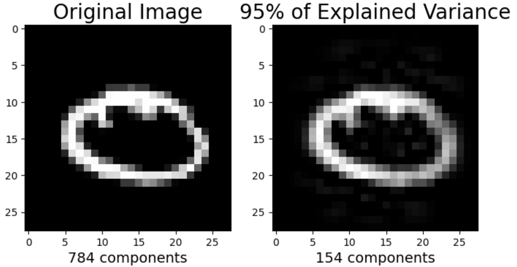
Now restore the sample to see the difference between the original picture and the original picture

approximation = model.inverse_transform(lower_dimensional_data) # Data Restoration after Dimension Reduction
plt.figure(figsize=(8,4));

# Original Picture
plt.subplot(1, 2, 1);
plt.imshow(X_train[1].reshape(28,28),
              cmap = plt.cm.gray, interpolation='nearest',
              clim=(0, 1));
plt.xlabel(f'{X_train.shape[1]} components', fontsize = 14)
plt.title('Original Image', fontsize = 20)
# Picture after dimension reduction
plt.subplot(1, 2, 2);
plt.imshow(approximation[1].reshape(28, 28),
              cmap = plt.cm.gray, interpolation='nearest',
              clim=(0,1));
plt.xlabel(f'{model.n_components_} components', fontsize = 14)
plt.title('95% of Explained Variance', fontsize = 20)
plt.show()

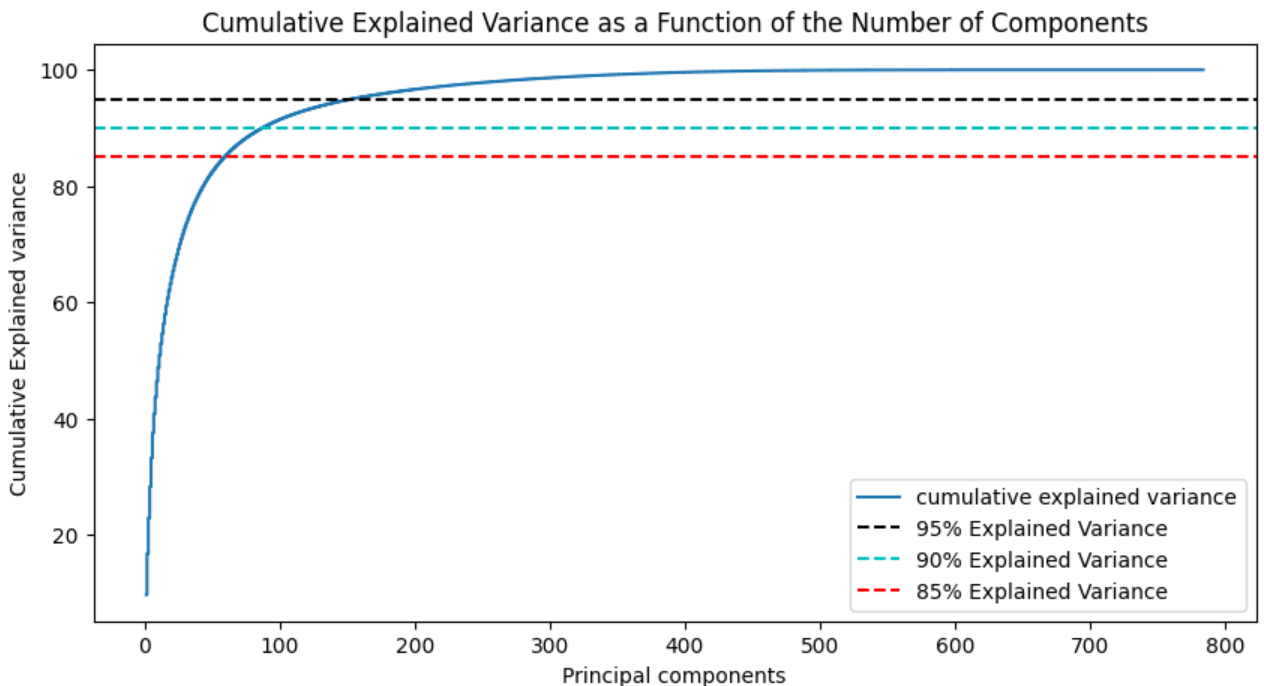
2.3. Explained Variance for the number of principal components

model = PCA() # You need to analyze all the principal components here, so don't reduce the dimensions
model.fit(X_train)
tot = sum(model.explained_variance_) 
var_exp = [(i/tot)*100 for i in sorted(model.explained_variance_, reverse=True)] 
cum_var_exp = np.cumsum(var_exp)
plt.figure(figsize=(10, 5))
plt.step(range(1, p+1), cum_var_exp, where='mid',label='cumulative explained variance') # p: number of characteristic dimensions
plt.title('Cumulative Explained Variance as a Function of the Number of Components')
plt.ylabel('Cumulative Explained variance')
plt.xlabel('Principal components')
plt.axhline(y = 95, color='k', linestyle='--', label = '95% Explained Variance')
plt.axhline(y = 90, color='c', linestyle='--', label = '90% Explained Variance')
plt.axhline(y = 85, color='r', linestyle='--', label = '85% Explained Variance')
plt.legend(loc='best')
plt.show()

def explained_variance(percentage, images): 
    '''
       :param: percentage [float]: Percentage of dimension reduction
       :return: approx_original: Pictures restored after dimension reduction
       :return: model.n_components_: Number of principal components after dimension reduction
    '''   
    model = PCA(percentage)
    model.fit(images)
    components = model.transform(images)
    approx_original = model.inverse_transform(components)
    return approx_original,model.n_components_
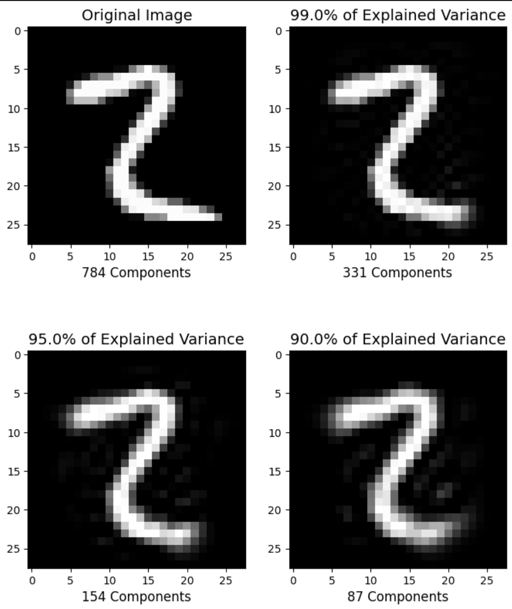
plt.figure(figsize=(8,10));
percentages = [784,0.99,0.95,0.90]
for i in range(1,5):
    plt.subplot(2,2,i)
    im, n_components = explained_variance(percentages[i-1], X_train)
    im = im[5].reshape(28, 28) # Rebuild to Picture
    plt.imshow(im,cmap = plt.cm.gray, interpolation='nearest',clim=(0,1))
    plt.xlabel(f'{n_components} Components', fontsize = 12)
    if i==1:
        plt.title('Original Image', fontsize = 14)
    else:
        plt.title(f'{percentages[i-1]*100}% of Explained Variance', fontsize = 14)
plt.show()

3. Summary

PCA calculates the principal components by selecting the dimension that maximizes the variance of the samples. After determining the direction vector of the principal components, you need to map the high-dimensional data to the low-dimensional data. The method is to multiply the sample points by each principal component vector (number) to get the number of k and form the vectors, and so on, to complete the mapping of high-dimensional n to low-dimensional k. The formula is: X ⋅ W k T = X k X \cdot W_{k}^{T}=X_{k} X⋅WkT​=Xk​

When we use the improved PCA method in sklearn, Instance object needs to be initialized first (The number of principal components can be passed in at this time), then the fit operation gets the principal components and then the dimension-reduction mapping operation pca.transform is performed. When initializing the instance object, a number can also be passed in indicating the proportion of variance explained by the principal components, that is, the importance of each principal component to the variance of the original data. Components that have little influence on the original variance are ignored and a weight is given between time and accuracy. Balance.