abstract

SMOTE is a synthetic data algorithm for comprehensive sampling, which is used to solve the unbalanced class problem and synthesize data by combining a few over sampling classes and most under sampling classes. This article will take Nitesh V. Chawla(2002) This paper expounds the core idea of SMOTE and its naive algorithm, compares the performance of the algorithm on the traditional classifier (Bayesian and decision tree), and discusses the ways to improve the algorithm.

1. Introduction

Class imbalance is one of the common problems in classifier model training, such as learning to judge whether a person has cancer through a large number of chest X-ray images, or learning to detect data patterns that may be aggressive behavior in network flow logs. There are more normal classes than abnormal classes (diagnosis belongs to cancer and aggressive behavior), The classifier trained under category unbalanced data should be very careful, even if the classifier has high accuracy, because it is likely to learn that most of them are normal, and what we may need is that it can identify abnormal behavior to the greatest extent, even if the accuracy is lower than the former.

In order to solve this problem, there are five recognized methods in the industry to expand the data set [1], so that the categories are uniform:

1. Randomly increase the number of samples of a few classes.
2. Randomly increase the number of specific minority samples.
3. Randomly reduce the number of samples of most classes.
4. Randomly reduce the number of samples of a specific majority class.
5. Modify the cost function to make the cost of a few class errors higher.

The SMOTE algorithm to be introduced in this paper is an improved way of synthesizing 1 and 3 methods. It randomly selects N adjacent points based on the k nearest neighbor sample points of each sample point, and multiplies the difference by a threshold in the range of [0,1], so as to achieve the purpose of synthesizing data. The core of this algorithm is that the features of adjacent points in feature space are similar. It does not sample in the data space, but in the feature space, so its accuracy will be higher than the traditional sampling method. This is why SMOTE and its derived algorithms are still the mainstream sampling technology so far.

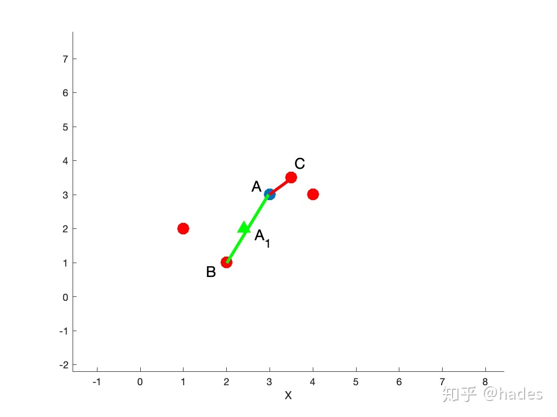
Figure 1

In Figure 1, it is assumed that data point a has four adjacent points in the feature space. If N is 2, SMOTE will randomly select two adjacent points B and C and calculate the distances of a - > b and a - > C respectively. As shown by the green line and red line in the figure, all sampling points on the green line or red line are reasonable, such as point A1. In order to ensure that the data points are as diverse as possible (without overlap), multiply by a random factor between [0,1].

In Chapter 2, the algorithm will be implemented according to the core of SMOTE and its pseudo code, and applied to the test data set; In Chapter 3, the SMOTE algorithm implemented in the third-party imbalanced learn library will be used for sampling to verify the accuracy of our algorithm. Of course, the algorithm in this library is better than the simple SMOTE algorithm. Later, we will use the decision tree and Gaussian Bayesian classifier as tools to test the original data Compare the performance of the data sets generated by SMOTE sampling and the data generated by the third-party library SMOTE; Chapter 4 will discuss the optimization approaches of more robust and better performance of naive SMOTE algorithm; Chapter 5 is the summary of this paper.

2. Algorithm analysis and Implementation

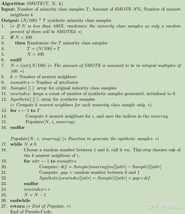
Fig. 2 is the pseudo code proposed in SMOTE paper, which is composed of two functions SMOTE(T, N, K) and Populate(N, i, nnarray).

Figure 2: algorithm

SMOTE is responsible for accepting the class data set X to be sampled and returning a data set sampled by SMOTE. The size is (N/100)*T. the function has three parameters, namely T: the number of samples of data set X to be processed; N: The sampling proportion is generally 100, 200, 300 and other hundreds, corresponding to 1, 2 and 3 times; K: Is the number of nearest neighbors sampled, which is 5 by default in the paper. The SMOTE code idea is very simple. Scan each sample point, calculate the k nearest neighbors of each sample point, record the index of each nearest neighbor sample point in nnarray, and then transfer it to Populate(N, i, nnarray), that is, complete the sampling of a sample point.

Populate is responsible for randomly generating N samples similar to observation sample i according to the index in nnarray. This function will calculate the difference dif between the random adjacent point nn and each feature of the observation sample i point, multiply the difference by a [0,1] random factor gap, and then add the value of dif*gap to the observation point i to complete the synthesis of a feature.

The implementation in Python is as follows:

Note: in order to ensure the reproducibility of all codes in this article, set random_state is 666

def NaiveSMOTE(X, N=100, K=5):
    """
    {X}: minority class samples;
    {N}: Amount of SMOTE; default 100;
    {K} Number of nearest; default 5;
    """
    # {T}: Number of minority class samples; 
    T = X.shape[0]
    if N < 100:
        T = (N/100) * T
        N = 100
    N = (int)(N/100)

    numattrs = X.shape[1]
    samples = X[:T]
    neigh = NearestNeighbors(n_neighbors=K)
    neigh.fit(samples)
    Synthetic = np.zeros((T*N, numattrs))
    newindex = 0

    def Populate(N, i, nns, newindex):
        """
        Function to generate the synthetic samples.
        """
        for n in range(N):
            nn = np.random.randint(0, K)
            for attr in range(numattrs):
                dif = samples[nns[nn], attr] - samples[i, attr]
                gap = np.random.random()
                Synthetic[newindex, attr] = samples[i, attr] + gap*dif
            newindex += 1
        return newindex

    for i in range(T):
        nns = neigh.kneighbors([samples[i]], K, return_distance=False)
        newindex = Populate(N, i, nns[0], newindex)
    return Synthetic

The matrix operation is not used here, but completely reproduced in the way in the paper (so it is called NaiveSMOTE). The nearest neighbor calculation is completed by using the NearestNeighbors class provided by scikit learn.

Next, we use make in scikit learn_ Classification to generate test classification data sets and simulate unbalanced data. Of course, interested readers can also find the data sets used in the paper.

from sklearn.datasets import make_classification
X, y = make_classification(n_samples=500,
                           n_features=9,
                           n_redundant=3,
                           weights=(0.1, 0.9),
                           n_clusters_per_class=2,
                           random_state=666)   # For reproducibility
print(X.shape, y.shape)       # ((500, 9), (500,))

# Number of samples to view y 
print(view_y(y))              # class 0: 50  class 1: 450

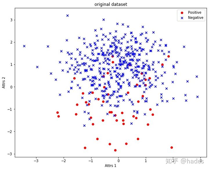
The distribution of the original data set is shown in Fig. 3, in which the red circle is a positive class, that is, a few classes, and blue × Is a negative class, that is, most classes.

Figure 3: original_dataset

Apply NaiveSMOTE we implemented to this test data:

X_over_sampling = NaiveSMOTE(X[y==0], N=800)
print(X_over_sampling.shape)         # (400, 9) 400 samples were added

# Merge the composite data with the original data set
new_X = np.r_[X, X_over_sampling]
new_y = np.r_[y, np.zeros((X_over_sampling.shape[0]))]
print(new_X.shape, new_y.shape)      # ((900, 9), (900,))

print(view_y(new_y))                 # class 0: 450 class 1: 450

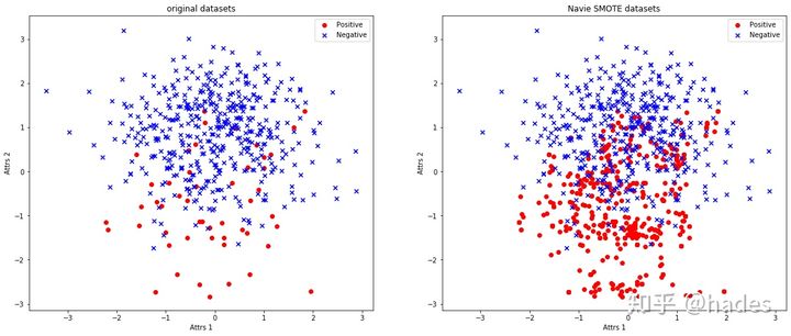
Next, we compare the original data set with the data set synthesized by NaiveSMOTE:

You can clearly see that the original class has increased to a satisfactory level, and the distance between the generated classes is not far.

Extension:

Explore SMOTE algorithm - Zhihu (zhihu.com)

SMOTE - wqbin - blog Park of oversampling algorithm (cnblogs.com)