[source code analysis] how Facebook trains super large models---

[source code analysis] how Facebook trains super large models -- (4)

0x00 summary

As we mentioned earlier, Microsoft ZeRO can expand a trillion parameter model on 4096 NVIDIA A100 GPU s using 8-way model parallel, 64-way pipeline parallel and 8-way data parallel. FSDP (full sharded data parallel) is an upgraded version of PyTorch DDP proposed by Facebook after deeply learning from Microsoft ZeRO. It can be regarded as benchmarking Microsoft ZeRO, and its essence is parameter sharding. Parameter sharding is to divide model parameters into GPUs. We will use Google, Microsoft and Facebook papers, blogs and code for learning and analysis.

In the previous article, we mentioned that FSDP supports mixed accuracy training, so let's take a look at the relevant knowledge.

Other articles in this series are as follows:

[Source code analysis] PyTorch distributed ZeroRedundancyOptimizer

[ZeRO of distributed training Parameter sharding

[Google Weight Sharding of distributed training Parameter Sharding

[Source code analysis] how Facebook trains super large models -- - (1)

[[source code analysis] how Facebook trains super large models -- - (2)

[[source code analysis] how Facebook trains super large models -- - (3)

0x01 background knowledge

1.1 differences between single precision, double precision and half precision floating point formats

We are from NVIDIA official blog What's the Difference Between Single-, Double-, Multi- and Mixed-Precision Computing? Excerpts are as follows:

IEEE floating point arithmetic standard is a general convention for representing numbers in binary on computers. In the double format, each number occupies 64 bits. The single precision format uses 32 bits, while the half precision is only 16 bits.

In traditional scientific notation, pi is written as 3.14 x \(10^0 \). However, the computer stores this information in binary form as floating-point numbers, that is, a series of 1 and 0 representing the number and its corresponding exponent, which in this case is 1.1001001 x\(2^1 \).

In single precision 32-bit format, one bit is used to determine whether a number is positive or negative. Eight bits are reserved for the exponent, which (because it is binary) is a power of 2. The remaining 23 bits are used to represent the numbers that make up the numbers, which are called significant numbers.

On the contrary, double precision reserves 11 bits for index and 52 bits for significant number, which greatly expands the range and size of numbers it can represent. Half precision takes up a smaller part, with only 5 bits for the index and 10 bits for the significant number.

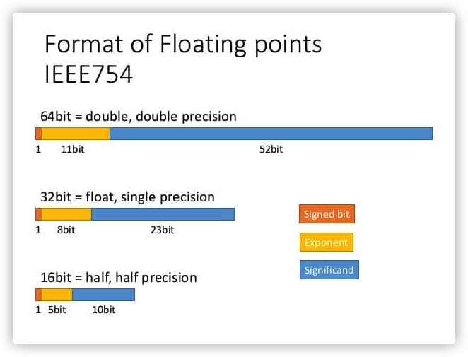
Here is what pi looks like at each precision level

1.2 difference between multi precision and mixed precision calculation

Multi precision computing means using processors that can calculate with different precision - semi precision or single precision algorithms that use double precision when needed and depend on other parts of the application.

Mixed accuracy, also known as super accuracy, is calculated by using different accuracy levels in a single operation to achieve computational efficiency without sacrificing accuracy. In mixed precision, the calculation starts with the half precision value of fast matrix mathematics. However, with the calculation of numbers, the machine stores the results with higher accuracy. For example, if you multiply two 16 bit matrices, the answer size is 32 bits.

Using this method, when the application completes the calculation, the cumulative answer is comparable in accuracy to running the whole thing in double precision arithmetic. This technology can increase the speed of traditional double precision applications by up to 25 times, while reducing the memory, running time and power consumption required to run them. It can be used for AI and simulated HPC workloads.

1.3 mixing accuracy

The advantages of FP16 are as follows:

Less memory. If FP16 is adopted, the model occupation is half that of FP32. In this way, a larger model can be trained, a larger batch size can be used, and the traffic is less.
Faster calculation. The accelerated optimization of FP16 can speed up the calculation of training and reasoning.
In addition, with the popularity of NVIDIA Tensor Core, FP6 computing is getting faster and faster.

The main problem with FP16 is that its representation range is narrower than FP32, so it will bring two problems: overflow error and rounding error. Therefore, Baidu and NVIDIA jointly put forward some technologies in the paper.

Keep a primary copy of the weight in FP32 format.
Use loss scale to prevent the ladder from being too small.
FP16 is used for calculation, but FP32 is used for accumulation.

For example, for primary backup, the legend in the paper is as follows:

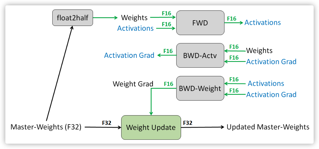
1.4 training process

The three techniques described above are a good supplement to the training process. We learn from the official NVIDIA documents https://docs.nvidia.com/deeplearning/performance/mixed-precision-training/index.html The training process is as follows.

Maintain a master copy of FP32 parameters.
For each iteration:
1. Make an FP16 copy of the weight.
2. Forward propagation using FP16 weights and activation.
3. Multiply the resulting loss by the scale factor S.
4. Using FP16 weights, activation and their gradients are propagated backward.
5. Multiply the weight gradient by 1/S.
6. Complete the weight update (including gradient client, etc.).

A more robust approach is to dynamically select the loss scale factor. The basic idea is to start with a large scale factor, and then reconsider it in each training iteration. If no overflow occurs in the selected number of iterations N, increase the scale factor. If overflow occurs, the weight update is skipped and the scale factor is reduced. We found that as long as we skip updates infrequently, the training plan does not need to be adjusted, and the same accuracy as FP32 training can be achieved.

Note that N effectively limits how often we can overflow and skip updates. The update rate of the scaling factor can be adjusted by selecting the increase / decrease multiplier and N (number of non overflow iterations before increase).

The dynamic loss scaling method corresponds to the following training process:

Keep a master copy of the weight in FP32.
Initialize S to a large value.
For each iteration
1. Make an FP16 copy of the weight.
2. Forward propagation (FP16 weight and activation).
3. Multiply the loss by the scale factor S.
4. Backward propagation (FP16 weights, activation and their gradients).
5. If there is Inf or NaN in the weight gradient.
  1. Reduce S.
  2. Skip the weight update and enter the next iteration.
6. Multiply the weight gradient by 1/S.
7. Complete weight update (including gradient clipping, etc.).
8. If Inf or NaN does not appear in the past N iterations, increase S.

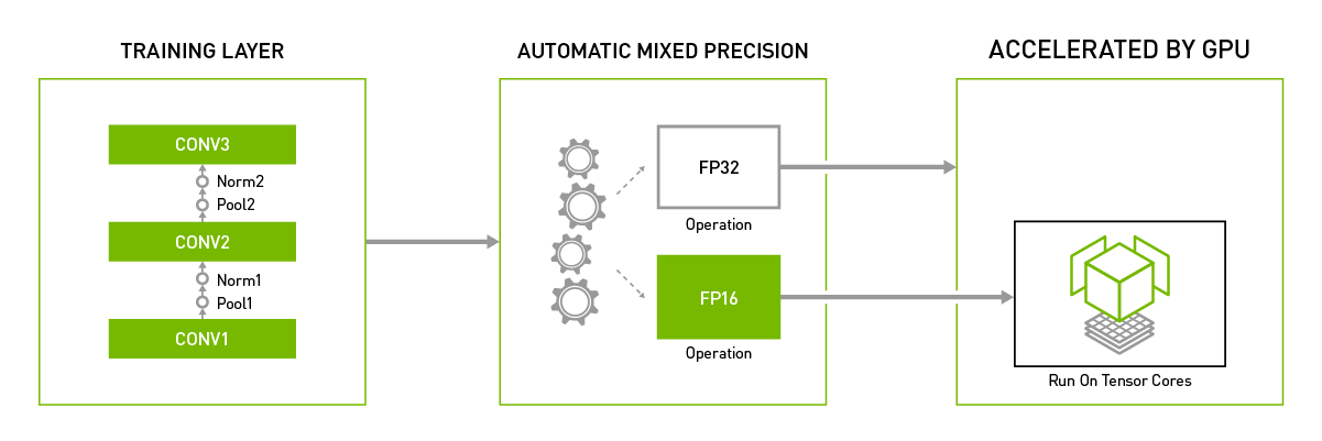
Picture from https://developer.nvidia.com/automatic-mixed-precision

0x02 PyTorch

2.1 NVIDIA computing power

The characteristics of NVIDIA's Volta and Turing GPU in FP16 computing are as follows:

The memory bandwidth and storage requirements of FP16 can be reduced by half compared with FP32, so that developers can use larger and more complex models and larger batch size under the same hardware conditions.
NVIDIA Volta and Turing architecture GPU provide Tensor Cores technology. The FP16 computing throughput of Tensor Cores is 8 times that of FP32.

Therefore, under the same super parameters, the mixed precision training using half precision floating point (FP16) and single precision (FP32) floating point can achieve the same accuracy as the pure single precision (FP32) training, and the model training speed can be greatly accelerated.

2.2 Torch.cuda.amp

The mixing accuracy in PyTorch mainly depends on torch cuda. Amp this library, which shows that this function is dependent on CUDA.

The previous analysis mentioned the reasons for mixed calculation because:

In some cases, it is not sensitive to the accuracy loss. The local accuracy loss has a very weak impact on the final training effect, and it can be accelerated by Tensor Cores. At this time, FP16 has an advantage.
In some cases, it is particularly sensitive to accuracy loss, and FP32 has advantages at this time.

In PyTorch, the tensor related to mixing accuracy is torch Floattensor and torch Halftensor, when the two are mixed together, it is the mixing accuracy. The framework will automatically (sometimes manually) adjust the type of a tensor according to the actual needs. In torch Floattensor and torch This is the reason for automatic mixed precision (AMP).

2.2.1 use

Specifically, PyTorch uses autocast + GradScaler. We from https://github.com/NVIDIA/DeepLearningExamples Find out the official examples.

The function of GradScaler is to enlarge the loss and prevent the gradient underflow, but this is only used when the gradient is transmitted by back propagation. When updating the weight, you also need to scale the gradient back to its original size.

autocast context should only include forward propagation and loss calculation, because back propagation will automatically use the same type of forward propagation.

from torch.cuda.amp import autocast as autocast

def do_train(
    model,
    data_loader,
    optimizer,
    scheduler,
    checkpointer,
    device,
    checkpoint_period,
    arguments,
    use_amp,
    cfg,
    dllogger,
    per_iter_end_callback_fn=None,
):
    # The default model is torch FloatTensor
    max_iter = len(data_loader)
    start_iter = arguments["iteration"]
    model.train()

    if use_amp:
        # Building GradScaler
        scaler = torch.cuda.amp.GradScaler(init_scale=8192.0)
    for iteration, (images, targets, _) in enumerate(data_loader, start_iter):
        iteration = iteration + 1
        images = images.to(device)
        targets = [target.to(device) for target in targets]

        if use_amp:
            with torch.cuda.amp.autocast(): # Forward propagation enable autocast
                loss_dict = model(images, targets)
        else:
            loss_dict = model(images, targets)

        losses = sum(loss for loss in loss_dict.values())

        # reduce losses over all GPUs for logging purposes
        loss_dict_reduced = reduce_loss_dict(loss_dict)
        losses_reduced = sum(loss for loss in loss_dict_reduced.values())

        # Note: If mixed precision is not used, this ends up doing nothing
        # Otherwise apply loss scaling for mixed-precision recipe
        if use_amp:        
            scaler.scale(losses).backward() # Amplification gradient
        else:
            losses.backward()

        def _take_step():
            if use_amp:
                scaler.step(optimizer) # Within the method, if the gradient is normal, update the weight, otherwise ignore this update
                scaler.update() # Do you need to increase the scaler
            else:
                optimizer.step()
            scheduler.step()
            optimizer.zero_grad()
        
        if not cfg.SOLVER.ACCUMULATE_GRAD:
            _take_step()
        else:
            if (iteration + 1) % cfg.SOLVER.ACCUMULATE_STEPS == 0:
                for param in model.parameters():
                    if param.grad is not None:
                        param.grad.data.div_(cfg.SOLVER.ACCUMULATE_STEPS)
                _take_step()

2.2.2 multiple models, losses and optimizers

If your network has multiple losses, you must call scaler separately in each network scale. If the network has multiple optimizers, you can call scaler alone in any of them Unscale, and you must call scaler separately in each step.

However, after all optimizers have completed the step operation in the iteration, scaler can be called Update, and can only be called once.

Each optimizer checks whether the gradient is infs/NaN and independently decides whether to skip this step. This may cause one optimizer to skip this step while the other does not. This should not hinder convergence, since skip steps rarely occur (possibly only once every hundreds of iterations).

scaler = torch.cuda.amp.GradScaler()

for epoch in epochs:
    for input, target in data:
        optimizer0.zero_grad()
        optimizer1.zero_grad()
        with autocast():
            output0 = model0(input)
            output1 = model1(input)
            loss0 = loss_fn(2 * output0 + 3 * output1, target)
            loss1 = loss_fn(3 * output0 - 5 * output1, target)

        # (retain_graph here is unrelated to amp, it's present because in this
        # example, both backward() calls share some sections of graph.)
        scaler.scale(loss0).backward(retain_graph=True)
        scaler.scale(loss1).backward()

        # You can choose which optimizers receive explicit unscaling, if you
        # want to inspect or modify the gradients of the params they own.
        scaler.unscale_(optimizer0)

        scaler.step(optimizer0)
        scaler.step(optimizer1)

        scaler.update()

2.2.3 distributed

torch.nn.DataParallel generates a thread on each device to run forward delivery. autocast state is thread local, so the following will not work:

model = MyModel()
dp_model = nn.DataParallel(model)

# Sets autocast in the main thread
with autocast():
    # dp_model's internal threads won't autocast.  The main thread's autocast state has no effect.
    output = dp_model(input)
    # loss_fn still autocasts, but it's too late...
    loss = loss_fn(output)

The repair is simple. In mymodel Use autocast in forward.

MyModel(nn.Module):
    ...
    @autocast()
    def forward(self, input):
       ...

# Alternatively
MyModel(nn.Module):
    ...
    def forward(self, input):
        with autocast():
            ...

The following code is in DP_ Automatic conversion between the thread of model (executing forward) and the main thread (executing loss_fn):

model = MyModel()
dp_model = nn.DataParallel(model)

with autocast():
    output = dp_model(input)
    loss = loss_fn(output)

torch. nn. parallel. The distributed data parallel documentation recommends that each process use a GPU for optimal performance. In this case, DistributedDataParallel will not generate threads internally, so the use of autocast and GradScaler will not be affected.

Or use with autocast() inside the forward method to ensure that autocast takes effect inside the process, for example.

def _forward(self, sample):
    loss = None
    oom = 0
    try:
        if sample is not None:
            with amp.autocast(enabled=self.args.amp):
                # calculate loss and sample size
                logits, _ = self.model(**sample['net_input'])
                target = sample['target']
                probs = F.log_softmax(logits, dim=-1, dtype=torch.float32)
                loss = self.criterion(probs, target)
    except RuntimeError as e:
        if 'out of memory' in str(e):
            print('| WARNING: ran out of memory in worker {}, skipping batch'.format(
                self.args.distributed_rank), force=True)
            oom = 1
            loss = None
        else:
            raise e
    return loss, oom

0x03 FSDP usage

torch.cuda.amp.autocast is fully compatible with FSDP, but users need to mix it_ Set precision to True. The specific example code is as follows:

offload_model = OffloadModel(
    model=model,
    device=torch.device("cuda"),
    offload_device=torch.device("cpu"),
    num_slices=3,
    checkpoint_activation=True,
    num_microbatches=1,
)

torch.cuda.set_device(0)
device = torch.device("cuda")

criterion = torch.nn.CrossEntropyLoss()
optimizer = torch.optim.SGD(offload_model.parameters(), lr=0.001)

# To train 1 epoch.
offload_model.train()
for batch_inputs, batch_outputs in dataloader:
    batch_inputs, batch_outputs = batch_inputs.to("cuda"), batch_outputs.to("cuda")
    start = time.time_ns()
    optimizer.zero_grad()
    inputs = batch_inputs.reshape(-1, num_inputs * num_inputs)
    
    with torch.cuda.amp.autocast(): # Set amp
        output = model(inputs)
        loss = criterion(output, target=batch_outputs)
        loss.backward()
    optimizer.step()

Let's take a look at the relevant source code of FSDP,

3.1 member variables

Because CPU offload and partition and other factors are involved, FSDP cannot simply use amp. It needs to be combined with CPU offload and partition. For example, FP16 parameter also needs partition and offload. Because amp will not automatically partition and offload, FSDP needs to take over this part of the work and explicitly switch part of the work.

The previous code mentioned some member variables related to mixed accuracy training. Here, the 32-bit and 16 bit parameters are partitioned respectively, and the offload operation will be performed accordingly.

_ fp32_shard: single parameter slicing of full precision (usually fp32, but this depends on the model data type passed in by the user). This can be done on the CPU or GPU, depending on the CPU_ Value of offload.
_ fp16_shard: in mixed accuracy mode, we maintain a parameter slice with reduced accuracy (usually fp16) on the computing device to perform calculation in forward / backward transfer. This is``_ fp16_shard, if mixed_precision is True `, which will be a single shard of parameters in fp16 for all gather.
_ full_param_padded: all weights used for calculation in forward and backward propagation (filled to be evenly divisible by world_size). This will resize in place and materialize only when needed (via all gather).

Corresponding settings need to be made in the code. If we plan to keep the FP32/FP16 parameters on the CPU, the fixed memory allows us to use non blocking transmission when moving the FP32/FP16 parameter fragments to the computing device in the future. Partition operations are handled uniformly by FP32 and FP16.

3.2 Scaler

In the Scaler method, FSDP has also launched a distinctive ShardedGradScaler. The actual use of PyTorch automatic mixing accuracy will depend on whether OSS is used with DDP or shardeddp.

If OSS is used with DDP, the normal PyTorch GradScaler can be used without any changes.
If OSS is used with shardeddp (to obtain gradient segmentation), a very similar process can be used, but it requires a gradient aware GradScaler. It can be found in fairscale optim. grad_ Used in scaler.

In both cases, Autocast can be used as usual, and the loss will be scaled and processed in the same way.

When we look at the ShardedGradScaler code, we will find that it is characterized by the use of dist.all_reduce regulates between ranges.

import torch
from torch.cuda.amp import GradScaler as TorchGradScaler
import torch.distributed as dist
from torch.optim import Optimizer

from .oss import OSS


class GradScaler(TorchGradScaler):
    def _unscale_grads_(
        self, optimizer: Optimizer, inv_scale: torch.Tensor, found_inf: torch.Tensor, allow_fp16: bool
    ) -> Dict[torch.device, torch.Tensor]:
        return super()._unscale_grads_(optimizer, inv_scale, found_inf, True)


class ShardedGradScaler(TorchGradScaler):
    """
    A shard-aware :class:`GradScaler<torch.cuda.amp.GradScaler>`, to be used in conjunction with
    :class:`OSS` and :class:`ShardedOptimizer`.

    Interface and usecases are not changed, more explanations can be found in the corresponding pytorch
    documentation https://pytorch.org/docs/stable/amp.html#torch.cuda.amp.GradScaler
    """

    def __init__(
        self,
        init_scale: float = 2.0 ** 16,
        growth_factor: float = 2.0,
        backoff_factor: float = 0.5,
        growth_interval: int = 2000,
        enabled: bool = True,
        process_group: Any = dist.group.WORLD,
    ) -> None:
        super().__init__(
            init_scale=init_scale,
            growth_factor=growth_factor,
            backoff_factor=backoff_factor,
            growth_interval=growth_interval,
            enabled=enabled,
        )
        self.display_warning = True
        self.group = process_group

    def unscale_(self, optimizer: Optimizer) -> None:
        # Could be a mistake, this scaler is supposed to work with ZeroRedundancyOptimizer only
        if self.display_warning and not isinstance(optimizer, OSS):
            logging.warning(
                "ShardedGradScaler is to be used in combination with a sharded optimizer, this could not be checked"
            )
        self.display_warning = False  # Only warn once

        # Call the upstream unscale_ method which will only act on this rank's gradients
        super().unscale_(optimizer)

        # Synchronize the detected inf across the ranks
        optimizer_state = self._per_optimizer_states[id(optimizer)]
        last_handle = None
        
        # AllReduce is used
        for v in optimizer_state["found_inf_per_device"].values():
            last_handle = dist.all_reduce(v, async_op=True, group=self.group)

        # Make sure that the calls are done before moving out.
        # The calls are executed in sequence, waiting for the last one is enough
        if last_handle is not None:
            last_handle.wait()

3.3 initialization

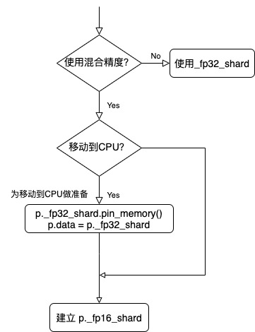
Let's then look at how offload and blending accuracy are used. In initialization method_ init_ param_ In attributes, there are also operations that will prepare for moving to the CPU, such as putting it into the lock page memory, and creating tensors for mixed accuracy, such as_ fp16_shard.

@torch.no_grad()
def _init_param_attributes(self, p: Parameter) -> None:

    if hasattr(p, "_fp32_shard"):
        return

    # A single shard of the parameters in full precision.
    p._fp32_shard = p.data

    if self.mixed_precision:

        # Prepare for move to CPU
        if self.move_params_to_cpu:
            # If we plan to keep the FP32 parameters on CPU, then pinning
            # memory allows us to later use non-blocking transfers when moving
            # the FP32 param shard to compute_device.
            p._fp32_shard = p._fp32_shard.pin_memory() 
            p.data = p._fp32_shard

        # In the mixed accuracy mode, we maintain a parameter slice with reduced accuracy (usually FP16) on the computing device,
        # Used to perform calculations in forward / backward passes.    
            
        # In mixed precision mode, we maintain a reduced precision
        # (typically FP16) parameter shard on compute_device for performing
        # the computation in the forward/backward pass. We resize the
        # storage to size 0 at init (here) and re-materialize (by copying
        # from _fp32_shard) as needed.
        p._fp16_shard = torch.zeros_like(p._fp32_shard, device=self.compute_device, dtype=self.compute_dtype)
        free_storage_(p._fp16_shard)
    else:
        p._fp16_shard = None  # use _fp32_shard

    # We also maintain a full-sized parameter of type self.compute_dtype
    # (FP16 for mixed_precision or FP32 otherwise). We resize the
    # storage to size 0 at init (here) and only materialize as needed. The
    # storage may contain padding elements so that it is evenly divisible by
    # world_size, although these padding elements will be removed before the
    # relevant computation.
    if p._is_sharded:
        p._full_param_padded = torch.zeros(
            p.data.numel() * self.world_size, device=self.compute_device, dtype=self.compute_dtype
        )
        free_storage_(p._full_param_padded)

    # Prepare for move to CPU     
        
    if self.move_grads_to_cpu: 
        # We can optionally move the grad shard to CPU during the backward
        # pass. In this case, it's important to pre-allocate the CPU grad
        # shard in pinned memory so that we can do a non-blocking transfer.
        p._cpu_grad = torch.zeros_like(p.data, device="cpu").pin_memory()

The logic is as follows:

3.4 reconstruction

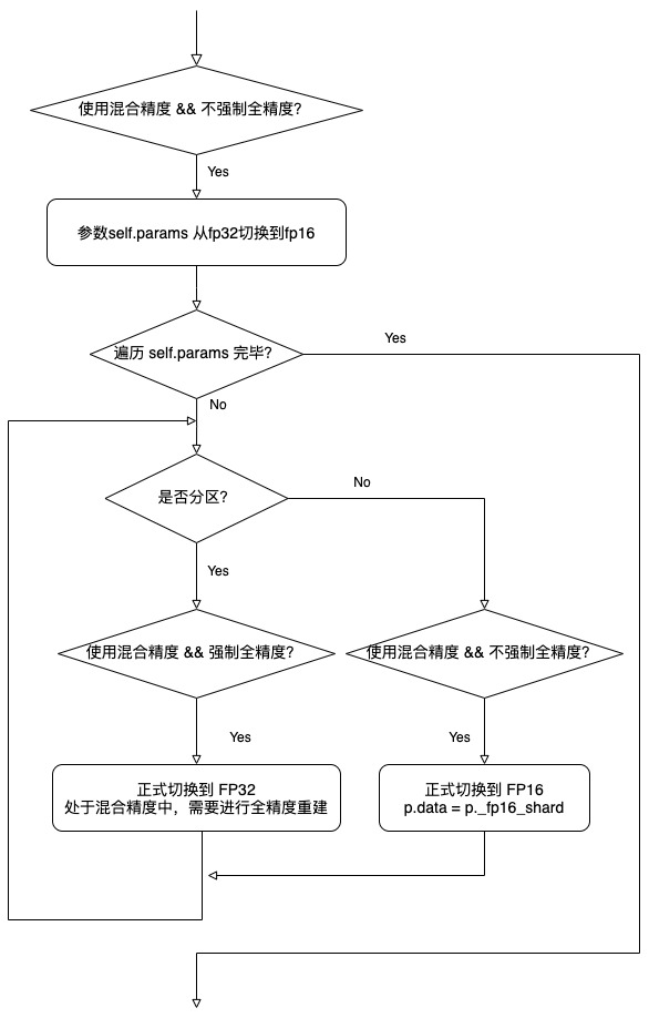
We take_ rebuild_full_params as an example. As previously analyzed, here is only an excerpt of the relevant code. The code will be switched according to various configurations. For example, if forced full precision is specified, it needs to be converted from FP16 to FP32, and then all gather.

@torch.no_grad()
def _rebuild_full_params(self, force_full_precision: bool = False) -> Optional[List[Tuple[torch.Tensor, bool]]]:

    output_tensors: List[Tuple[torch.Tensor, bool]] = []

    def update_p_data(custom_output_tensor: Optional[torch.Tensor] = None) -> None:
        """
        Helper function to update p.data pointer.
        """
        if custom_output_tensor is not None:
             # ellipsis
        elif not p._is_sharded:
            if self.mixed_precision and not force_full_precision: # Switch to FP16
                p.data = p._fp16_shard
                output_tensors.append((p.data, True))
            else:
                # Here p.data == p._fp32_shard, so it's not safe to free.
                output_tensors.append((p.data, False))
        else:
            # ellipsis
        # Trim any padding and reshape to match original size.
        p.data = p.data[: p._orig_size.numel()].view(p._orig_size)


    with torch.cuda.stream(self._streams["all_gather"]):
      
        if self.mixed_precision and not force_full_precision:
            self._cast_fp32_param_shards_to_fp16() # Switch from fp32 to fp16

        for p in self.params:
            if not p._is_sharded:  # e.g., when world_size == 1
                update_p_data()
            else:
                # If self.move_params_to_cpu and force_full_precision, we need to cast
                # the FP32 CPU param to CUDA for the all-gather.
                
                # Copy to GPU
                p_data = p.data.to(p._full_param_padded.device, non_blocking=True)

                p_size = p._full_param_padded.size()
                if self.mixed_precision and force_full_precision:
                    # Allocate fresh tensor in full precision since we are in
                    # mixed precision and full precision rebuild is asked.
                    
                    # Assign new tensors in full accuracy, because we are in mixed accuracy and need full accuracy reconstruction.
                    output_tensor = p_data.new_zeros(p_size)
                else:
                    if p._full_param_padded.storage().size() != p_size.numel():
                        alloc_storage_(p._full_param_padded, size=p_size)
                    output_tensor = p._full_param_padded

                # Fill output_tensor with (p.data for each shard in self.world_size)
                dist.all_gather(chunks, p_data, group=self.process_group) # Simplified version code

                if self.mixed_precision and not force_full_precision:
                    self._free_fp16_param_shard([p]) # Free memory
                    
                # ellipsis

The logic is as follows:

3.5 cast operation

Can from_ cast_ fp32_ param_ shards_ to_ See how to do conversion operation in fp16.

@torch.no_grad()
def _cast_fp32_param_shards_to_fp16(self, params: Optional[List[Parameter]] = None) -> None:
    """Cast FP32 param shard to FP16 for a list of params."""
    if params is None:
        params = self.params
    with torch.cuda.stream(self._streams["fp32_to_fp16"]):
        for p in params:
            alloc_storage_(p._fp16_shard, size=p._fp32_shard.size())
            p._fp16_shard.copy_(
                # If cpu_offload is True, this will be non-blocking because
                # _fp32_shard is pinned, otherwise it's a no-op.
                p._fp32_shard.to(p._fp16_shard.device, non_blocking=True)
            )
            p.data = p._fp16_shard
    torch.cuda.current_stream().wait_stream(self._streams["fp32_to_fp16"])

3.6 _post_reduction_hook

In_ post_ backward_ Callback will be set in hook_ FN is called after reduce-scatter. post_reduction_hook, understandably, is that after this operation, you can move the gradient to the CPU.

callback_fn = functools.partial(self._post_reduction_hook, param)

The specific code is as follows. Related to offload is the operation of moving the gradient to the CPU, and related to mixing accuracy is the conversion of the gradient to the type of parameter tensor.

def _post_reduction_hook(self, param: Parameter, reduced_grad: torch.Tensor) -> None:
    """Hook to call on each param after the reduce-scatter."""

    param.grad.data = reduced_grad
    if self.gradient_postdivide_factor > 1:
        # Average grad by world_size for consistency with PyTorch DDP.
        param.grad.data.div_(self.gradient_postdivide_factor)
        
    # Cast grad to param's dtype (typically FP32). Note: we do this
    # before the move_grads_to_cpu step so that this entire hook remains
    # non-blocking. The downside is a bit more D2H transfer in that case.
    if self.mixed_precision:
        orig_param_grad_data = param.grad.data # Convert the gradient, generally switch back to FP32
        param.grad.data = param.grad.data.to(dtype=param.data.dtype)
        # Don't let this memory get reused until after the transfer.
        orig_param_grad_data.record_stream(torch.cuda.current_stream())
        
    if hasattr(param, "_saved_grad_shard") and param._saved_grad_shard is not None:
        param.grad.data += param._saved_grad_shard
        delattr(param, "_saved_grad_shard")
        
    # Optionally move gradients to CPU, typically used if one is running
    # the optimizer on the CPU.
    if self.move_grads_to_cpu: # Move gradient to CPU
        param._cpu_grad.copy_(param.grad.data, non_blocking=True)
        # Don't let this memory get reused until after the transfer.
        param.grad.data.record_stream(torch.cuda.current_stream())
        param.grad.data = param._cpu_grad

So far, the mixing accuracy analysis is completed. Let's see how FSDP uses activation recommendation in the next article. Please look forward to it.