1. Adopt standard wav header and use code to read and write PCM WAV files.

The wave module in Python standard library is a convenient interface for audio wav format. The functions in this module can write audio data in the original format to files such as objects, and read the attributes of WAV files.
The wave module provides a convenient interface for processing WAV sound format. It does not support compression / decompression, but supports mono / stereo.
The contextlib module contains utilities for handling context managers and with statements.

#!/usr/bin/env python
# -*- coding:utf-8 -*-
# @FileName  :read_write_pcm_wav.py
# @Time      :2022/2/15 19:25
# @Author    :PangXZ
import wave
import contextlib
import numpy as np

"""
read test.wav，And convert it to PCM format
"""


def wav2pcm(wav_file, pcm_file):
    if wav_file is None or pcm_file is None:
        return
    with contextlib.closing(wave.open(wav_file, 'r')) as f:
        wav_params = f.getparams()
        ## wav_params: _wave_params(nchannels=, sampwidth=, framerate=, nframes=, comptype=,compname=)
        print('read WAV File:{}'.format(wav_file))
        print('Number of channels:{}'.format(wav_params[0]))
        print('Quantized digits:{}'.format(wav_params[1] * 8))
        # Quantization bits 1, 2 and 3 represent 8 bits, 16 bits and 24 bits respectively
        print('Sampling rate:{}'.format(wav_params[2]))
        print('Total number of samples:{}'.format(wav_params[3]))
        print('Audio duration:{}'.format(wav_params[3] / wav_params[2]))
        print('Compression format:{}'.format(wav_params[4]))

        # Read the sampling value and store it in bytes format
        wav_bytes = f.readframes(wav_params[3])
        # Convert to array
        wave_data = np.frombuffer(wav_bytes, dtype=np.int16)
        wave_data.tofile(pcm_file)
    print('convert wav to pcm finish.')


""":
read test.pcm Files, converting to WAV file"""


def pcm2wav(pcm_file, wav_file):
    if pcm_file is None or wav_file is None:
        return
    f = open(pcm_file, 'rb')
    pcm_bytes = f.read()
    with contextlib.closing(wave.open(wav_file, 'wb')) as f:
        # Add wav header and save it in wav format
        f.setframerate(16000)  # 16kHz (sampling frequency)
        f.setsampwidth(2)  # The quantization bits are divided into 8 bits, 16 bits and 24 bits
        f.setnchannels(1)  # Mono amplitude data bit n*1 matrix point, stereo is n*2 Matrix point
        f.writeframes(pcm_bytes)
    print('convert pcm to wav finish.')


if __name__ == "__main__":
    wav_name = 'test.wav'
    wav2pcm_name = 'test.pcm'
    wav2pcm(wav_name, wav2pcm_name)
    pcm2wav_name = 'pcm2wav_test.wav'
    pcm2wav(wav2pcm_name, pcm2wav_name)

2. Complete the code implementation of FBank, MFCC and PLP acoustic feature extraction

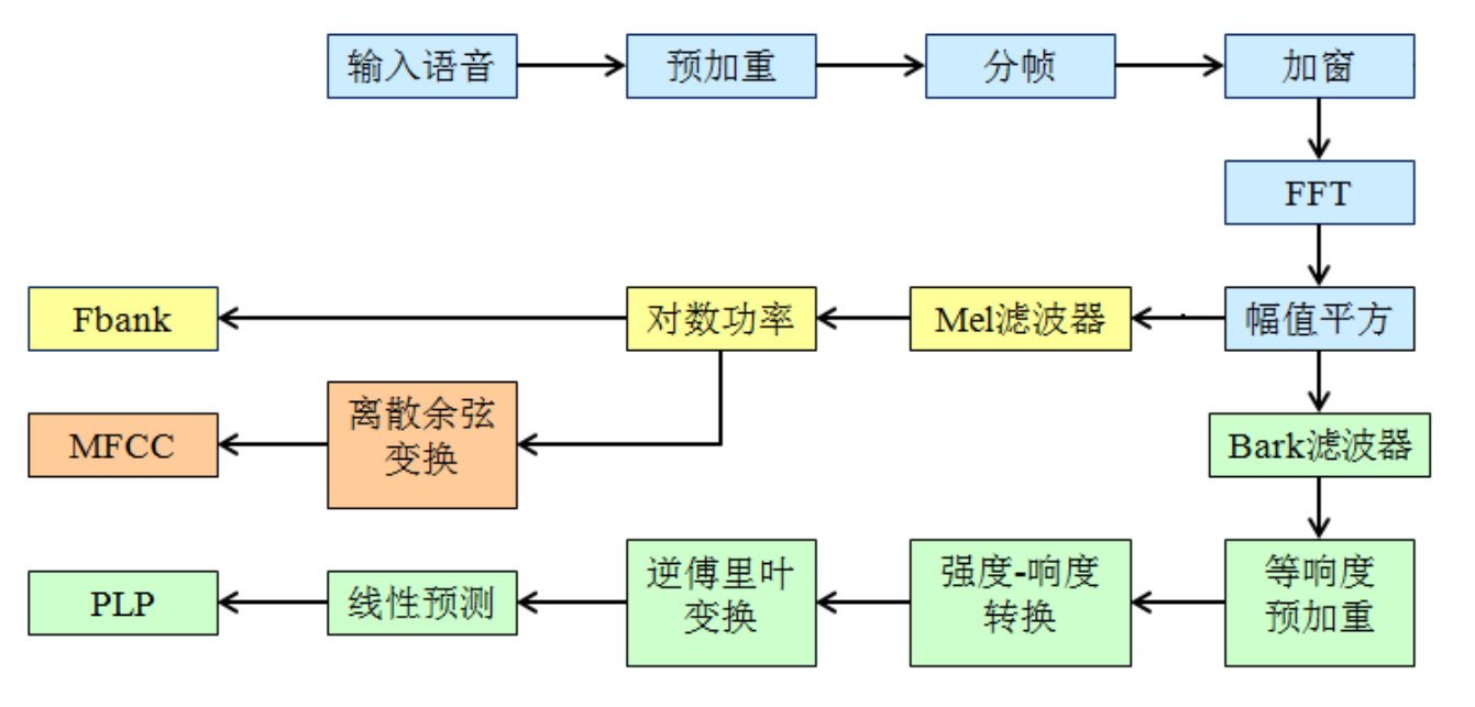
Fbank: (filter bank) the response of human ear to sound spectrum is nonlinear. Fbank is a front-end processing algorithm. Processing audio in a way similar to human ear can improve the performance of speech recognition. The general steps to obtain the fbank feature of speech signal are: pre emphasis, framing, windowing, short-time Fourier transform (STFT), power spectrum, amplitude square, Mel filter bank, logarithm, etc. MFCC features can be obtained by discrete cosine transform (DCT) of fbank.

MFCC (Mel frequency cepstral coefficients): Mel frequency cepstral coefficients. Mel frequency is proposed based on the auditory characteristics of human ears, which has a nonlinear correspondence with Hz frequency. Mel frequency cepstrum coefficient (MFCC) is the Hz spectrum characteristic calculated by using this relationship between them. It is mainly used for feature extraction of speech data and reduction of operation dimension. For example, for a frame with 512 dimensional (sampling point) data, the most important 40 dimensional (generally speaking) data can be extracted after MFCC, and the purpose of dimensionality reduction is also achieved.

PLP(Perceptual Linear Predictive coefficient) is a characteristic parameter based on Bark auditory model. It adopts the linear prediction method to realize the deconvolution processing of speech signal and obtain the corresponding acoustic characteristic parameters. It mainly includes: spectrum analysis, critical band analysis, zero loudness pre emphasis, intensity loudness conversion, inverse discrete Fourier transform, linear prediction and other steps.

Flow chart of speech feature extraction of Fbank, MFCC and PLP:

#!/usr/bin/env python
# -*- coding:utf-8 -*-
# @FileName  :Fbank_Processing.py
# @Time      :2022/2/15 20:44
# @Author    :PangXZ
import sys
import wave
import librosa
import contextlib
import numpy as np
import matplotlib.pyplot as plt

from scipy.io import wavfile
from scipy.fftpack import dct


def plot_time(sig, fs):
    '''
    Draw time domain diagram
    :param sig: speech signal 
    :param fs:  sampling period 
    :return:
    '''
    time = np.arange(0, len(sig)) * (1.0 / fs)
    plt.figure(figsize=(20, 5))
    plt.plot(time, sig)
    plt.xlabel('Times(s)')
    plt.ylabel('Amplitude(dB)')  # range
    plt.grid()
    plt.show()


def plot_freq(sig, sample_rate, nfft=512):
    '''
    Draw imperial concubines
    :param sig:
    :param sample_rate:
    :param nfft:
    :return:
    '''
    freqs = np.linspace(0, sample_rate / 2, nfft // 2 + 1)
    xf = np.fft.rfft(sig, nfft) / nfft
    xfp = 20 * np.log10(np.clip(np.abs(xf), 1e-20, 1e100))  # strength
    plt.figure(figsize=(20, 5))
    plt.plot(freqs, xfp)
    plt.xlabel('Freq(Hz)')
    plt.ylabel('Amplitude(dB)')  # strength
    plt.grid()
    plt.show()


def plot_spectrogram(spec, name):
    fig = plt.figure(figsize=(20, 5))
    heatmap = plt.pcolor(spec)
    fig.colorbar(mappable=heatmap)
    plt.xlabel('Times(s)')
    plt.ylabel('Frequency(Hz)')
    # tight_layout automatically adjusts the subgraph parameters to fill the entire image area
    plt.tight_layout()
    plt.title(name)
    plt.show()


# Define two formulas related to PLP: bark_change is linear frequency coordinate, converted to Bark coordinate, equal_loudness is equal loudness curve
def bark_change(x):
    return 6 * np.log10(x / (1200 * np.pi) + ((x / 1200 * np.pi)) ** 2 + 1) ** 0.5


def equal_loudness(x):
    return ((x ** 2 + 56.8e6) * x ** 4) / ((x ** 2 + 6.3e6) ** 2 * (x ** 2 + 3.8e8))


if __name__ == '__main__':
    # Data preparation
    wav_file = 'test.wav'
    sample_rate, signal = wavfile.read(wav_file)
    # sample_rate: is the sampling rate of the wav file, and signal is the content of the file, that is, the voice signal
    # View the number of channels of voice signal
    # print(f"number of channels = {signal.shape[1]}")
    # If wav is a dual channel, take the data of the first channel
    # signal = signal[:, 0]
    signal = signal[0: int(10 * sample_rate)]  # # Retain the first 10s data
    plot_time(signal, sample_rate)
    plot_freq(signal, sample_rate)

    # 1. Pre emphasis
    pre_emphasis = 0.97
    emphasized_signal = np.append(signal[0], signal[1:] - pre_emphasis * signal[:-1])
    plot_time(emphasized_signal, sample_rate)
    plot_freq(emphasized_signal, sample_rate)
    print('Dimension of voice signal:{}, Sampling rate:{}'.format(signal.shape, sample_rate))

    # 2. Framing
    frame_size, frame_stride = 0.025, 0.01  # The frame length is 25ms and the frame shift is 10ms
    frame_length, frame_step = int(round(frame_size * sample_rate)), int(round(frame_stride * sample_rate))
    signal_length = len(emphasized_signal)
    num_frame = int(np.ceil(np.abs(signal_length - frame_length) / frame_step)) + 1
    pad_signal_length = (num_frame - 1) * frame_step + frame_length
    pad_zero = np.zeros(int(pad_signal_length - signal_length))
    # If the number of points in the last frame after framing is insufficient, fill in zero
    pad_signal = np.append(emphasized_signal, pad_zero)
    # The following table for each frame
    indices = np.arange(0, frame_length).reshape(1, -1) + np.arange(0, num_frame * frame_step, frame_step).reshape(-1,
                                                                                                                   1)
    frames = pad_signal[indices]
    # frames is a two-dimensional array, each row is a frame, and the number of columns is the sampling points of each frame. The subsequent short-time fft operates directly on each column
    print('Dimension after framing:{}'.format(frames.shape))

    # 3. Add Hamming window
    hamming = np.hamming(frame_length)
    # hamming = 0.54 - 0.46 * np.cos(2 * np.pi * np.arange(0, frame_length) /(frame_length - 1))
    # Show windowing effect
    plt.figure(figsize=(20, 5))
    plt.plot(hamming)
    plt.grid()
    plt.xlim(0, 400)
    plt.ylim(0, 1)
    plt.xlabel('Samples')
    plt.ylabel('Amplitude')
    frames = frames * hamming
    plot_time(frames, sample_rate)
    plot_freq(frames.reshape(-1, ), sample_rate)
    print('Dimension after windowing:{}'.format(frames.reshape(-1, ).shape))

    # 4. Fast Fourier transform (FFT)
    NFFT = 512
    mag_frames = np.absolute(np.fft.rfft(frames, NFFT))  # Amplitude spectrum
    # 5. Power spectrum
    pow_frames = ((1.0 / NFFT) * (mag_frames ** 2))
    # Display power spectrum
    plt.figure(figsize=(20, 5))
    plt.plot(pow_frames[1])
    plt.grid()
    plt.show()

    # Fbank
    low_freq_mel = 0  # Minimum mel value
    high_freq_mel = 2595 * np.log10(1 + (sample_rate / 2.0) / 700)  # Maximum mel value and maximum signal frequency is fs/2
    print("Mel Upper cut-off frequency of filter:{}，Lower cut-off frequency:{}".format(low_freq_mel, high_freq_mel))
    nfilt = 40  # Number of filters
    mel_points = np.linspace(low_freq_mel, high_freq_mel, nfilt + 2)  # nfilt mel values are evenly distributed between the lowest and highest mel
    # For all mel center points, in order to facilitate the later calculation of mel filter bank, a center point is added on the left and right sides respectively
    hz_points = 700 * (10 ** (mel_points / 2595) - 1)  # mel value corresponds to the return frequency point, and the frequency interval is indexed
    fbank = np.zeros((nfilt, int(NFFT / 2 + 1)))  # Values of mel filters at corresponding points of energy spectrum

    bin = (hz_points / (sample_rate / 2)) * (NFFT / 2)  # The center point of each mel filter corresponds to the area code of FFT to find the position with value
    # Finding mel filter coefficients
    for i in range(1, nfilt + 1):
        left = int(bin[i - 1])  # Left boundary point
        center = int(bin[i])  # Center point
        right = int(bin[i + 1])  # Right boundary point
        for j in range(left, center):
            fbank[i - 1, j + 1] = (j + 1 - bin[i - 1]) / (bin[i] - bin[i - 1])
        for j in range(center, right):
            fbank[i - 1, j + 1] = (bin[i + 1] - (j + 1)) / (bin[i + 1] - bin[i])
    # mel filtering
    filter_banks = np.dot(pow_frames, fbank.T)
    filter_banks = np.where(filter_banks == 0, np.finfo(float).eps, filter_banks)
    # Take logarithm
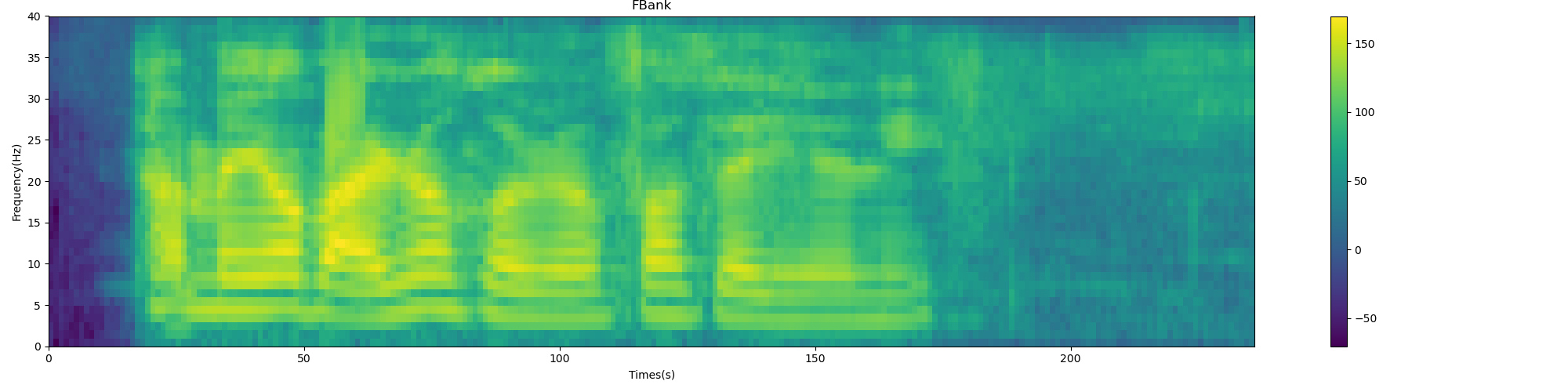
    filter_banks = 20 * np.log10(filter_banks)  # dB
    print('Shape of FBank: {}'.format(filter_banks.shape))
    plot_spectrogram(filter_banks.T, 'FBank')

    # MFCC
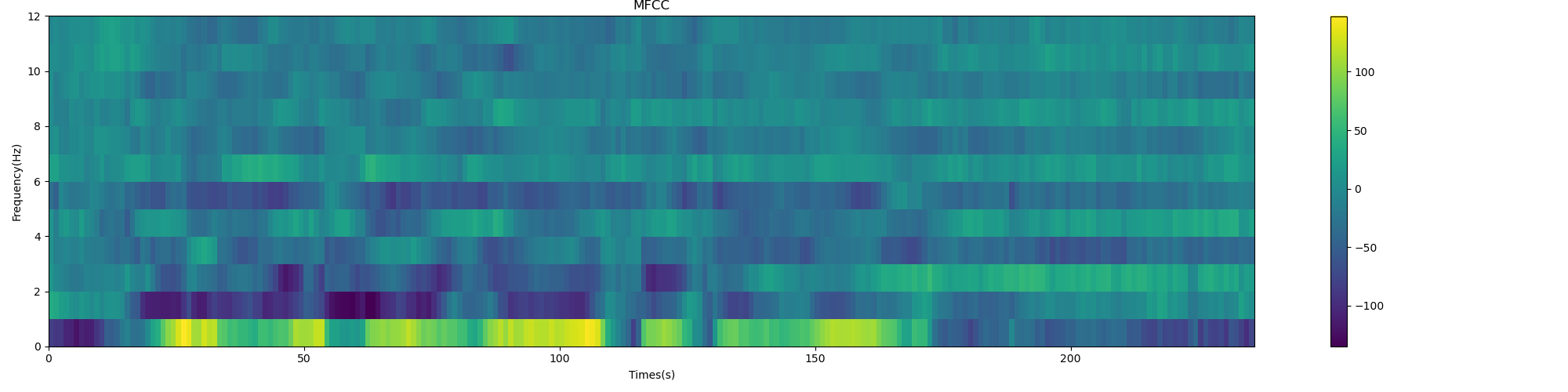
    num_ceps = 12  # Number of cepstrum coefficients retained
    mfcc = dct(filter_banks, type=2, axis=1, norm='ortho')[:, 1:(num_ceps + 1)]  # Keep at 2 ~ 13
    print("Shape of MFCC: {}".format(mfcc.shape))
    plot_spectrogram(mfcc.T, 'MFCC')

    # PLP
    N = int(NFFT / 2 + 1)
    df = sample_rate / N  # frequency resolution 
    i = np.arange(N)  # Only take the frequency greater than 0
    freq_hz = i * df  # Get the actual frequency coordinates: 0 - > sample_ rate

    freq_w = 2 * np.pi * np.array(freq_hz)  # Convert to angular frequency
    freq_bark = bark_change(freq_w)  # Then convert to bark frequency

    # The number of critical frequency bands selected is generally greater than 10, covering the common frequency range. Here, 15 central frequency points are selected
    point_hz = [250, 350, 450, 570, 700, 840, 1000, 1170, 1370, 1600, 1850, 2150, 2500, 2900, 3400]
    point_w = 2 * np.pi * np.array(point_hz)  # Convert to angular frequency
    point_bark = bark_change(point_w)  # Convert to bark frequency

    bank = np.zeros((15, N))  # Construct a matrix with 15 rows and 257 columns, and each row has a filter vector
    filter_data = np.zeros(15)  # 15 dimensional band construction energy vector
    # -------Critical band analysis: constructing filter banks---------
    for j in range(15):
        for k in range(N):
            omg = freq_bark[k] - point_bark[j]
            if -1.3 < omg < -0.5:
                bank[j, k] = 10 ** (2.5 * (omg + 0.5))
            elif -0.5 < omg < 0.5:
                bank[j, k] = 1
            elif 0.5 < omg < 2.5:
                bank[j, k] = 10 ** (-1.0 * (omg - 0.5))
            else:
                bank[j, k] = 0
    bark_filter_banks = np.dot(pow_frames, bank.T)

    # Equal loudness pre emphasis
    equal_data = equal_loudness(point_w) * bark_filter_banks

    # Intensity loudness conversion, which approximately simulates the nonlinear relationship between the intensity of sound and the loudness felt by human ears
    cubic_data = equal_data ** 0.33

    # Do the ifft (inverse Fourier transform) of 30 points to obtain the 30 dimensional PLP vector
    plp_data = np.fft.ifft(cubic_data, 30)

    # linear prediction
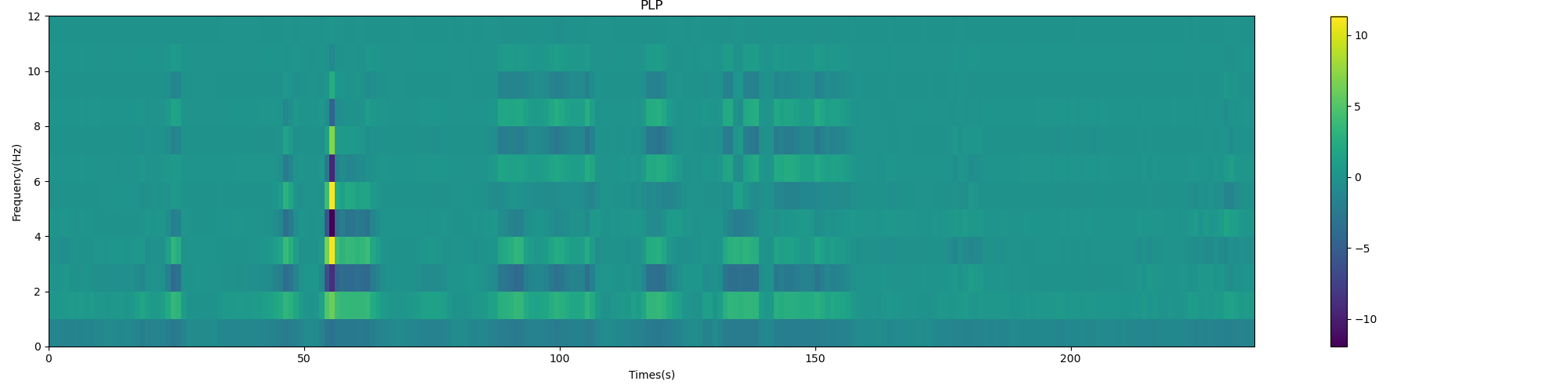
    plp = np.zeros((plp_data.shape[0], 12))
    for i in range(plp_data.shape[0]):
        plp[i] = librosa.lpc(abs(plp_data[i]), order=12)[1:]
    # print(plp,plp.shape)
    print("shape of PLP", plp.shape)
    plot_spectrogram(plp.T, 'PLP')

FBank spectrum:

MFCC spectrum:

PLP characteristic spectrum:

3. For MFCC, answer the following questions:

3.1 analyze the relationship between sampling rate, frame length, frame shift and the number of MFCC vectors.

• Sampling rate: refers to the number of sound wave amplitude samples per second when the analog sound waveform is digitized;
• Frame length: the speech signal has short-term stability, so the speech is divided into small segments (frames) for processing. This speech signal segment is a quasi steady-state process, generally about 10ms~30ms
• Frame shift: in order to avoid the excessive change of two adjacent frames, there will be an overlapping area between two adjacent frames. The overlapping area is obtained by a frame shift smaller than the frame length;
• Number of MFCC vectors: MFCC refers to the characteristics of each frame length range speech signal after analysis and processing. The number of vectors = the number of frames after framing

For example, the total duration of voice is 1.17s, the sampling rate is 16k, and the total sampling point is 1.17 × 16000 = 18720 1.17\times 16000 = 18720 one point one seven × 16000=18720； The frame length is 25ms, the frame shift is 10ms, and the number of MFCC vectors is ⌈ ( 1.17 − 0.025 ) / 0.01 ⌉ + 1 = 116 \lceil (1.17-0.025)/0.01 \rceil+1=116 ⌈(1.17−0.025)/0.01⌉+1=116

3.2 analyze the relationship between FFT size and sampling points per frame

The number of FFT points should be greater than the number of sampling points per frame (to prevent aliasing), which should generally be the nth power of 2, which is convenient for FFT to perform more levels of bisection, so as to speed up the transformation speed. For example, each frame has 512 L sampling points.

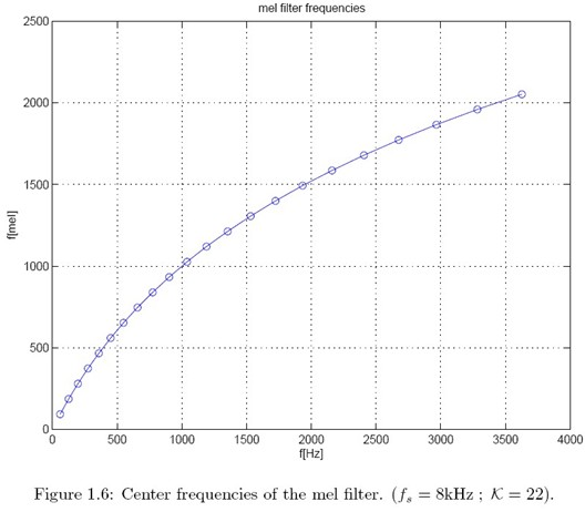
3.3 analyze the calculation process of Mel frequency

Mel frequency is a unit of tone, which is used to simulate the human ear's perception of speech at different frequencies. 1mel is equivalent to 1 / 1000 of the degree of 1kHz tone perception. The specific relationship between Mel frequency and actual frequency is as follows: m e l ( f ) = 2595 log ⁡ 1 + f 700 H z mel(f)=2595\log{1+\frac{f}{700Hz}} mel(f)=2595log1+700Hzf​
The auditory characteristics of human ear are consistent with the increase of Mel frequency. It shows a linear distribution with the actual frequency below 1000Hz and a logarithmic growth above 1000Hz.
Assuming that the sampling frequency of the speech signal is 8kHz, the frame length is N=256 and the number of filters is K=22, the maximum frequency of the speech signal can be obtained (according to Nyquist) f g = f s 2 = 4000 H z f_g=\frac{f_s}{2}=4000Hz fg​=2fs​​=4000Hz
According to the above formula, the maximum Mel frequency is: f m a x [ m e l ] = 2146.06 m e l f_max[mel]=2146.06 mel fm​ax[mel]=2146.06mel
Since the center frequency of each triangular filter is a linear distribution with equal intervals within the Mel scale range, the spacing between the center frequencies of two adjacent triangular filters can be calculated as: Δ m e l = f m a x [ m e l ] K + 1 = 93.3 m e l \Delta_{mel}=\frac{f_{max}[mel]}{K+1}=93.3 mel Δmel​=K+1fmax​[mel]​=93.3mel
Therefore, the center frequency of each triangular filter on mel scale can be expressed as m e l [ f ( m ) ] − m e l [ f ( m − 1 ) ] = m e l [ f ( m + 1 ) ] − m e l [ f ( m ) ] mel[f(m)]-mel[f(m-1)]=mel[f(m+1)]-mel[f(m)] mel[f(m)] − mel[f(m − 1)]=mel[f(m+1)] − mel[f(m)], the frequency on the corresponding linear scale can be calculated from the center frequency above. As shown in the figure below, the center frequency of mel is evenly distributed on the y axis, while on the x axis, the frequency interval of F center frequency becomes larger and larger with the increase of frequency.

3.4 analyze the static characteristics of MFCC obtained after DCT transformation

Discrete cosine transform (DCT) is a variant of Fourier transform. The advantage is that the result is real and has no imaginary part. DCT is also characterized by energy concentration, which can concentrate the signal energy on a very small number of transformation coefficients, especially the energy of most natural signals (including sound and image) can be concentrated in the low-frequency part after discrete cosine transform. The spectrum of speech signal can be regarded as formed by low-frequency envelope and high-frequency detail modulation.
For general speech signals, the first few coefficients of the result of this step are particularly large, and the latter coefficients are relatively small. In practice, only the first 13 ~ 20 are generally retained, which further compresses the data. Carry out cepstrum analysis on Mel spectrum (take logarithm and do inverse transform. The actual inverse transform is generally realized through DCT discrete cosine transform, and take the second to 13th coefficients after DCT as MFCC coefficients) to obtain Mel frequency cepstrum coefficient MFCC, which is the characteristic of this frame of speech; The low-frequency component of cepstrum is the envelope of spectrum, and the high-frequency component of cepstrum is the details of spectrum.
Of course, in the actual calculation of MFCC, we do not do the inverse Fourier transform, but first pass the spectrum through a group of triangular filters, and then do the discrete cosine transform (DCT) to obtain the MFCC coefficients. But its physical meaning is the same, that is, the distribution of the energy of the signal spectrum in different frequency ranges. The function of each filter is to obtain the spectral energy of the corresponding frequency range. If we have 26 triangular filters, we will get 26 MFCC coefficients. At this time, the lower coefficients can represent the characteristics of the channel.

3.5 calculation process of analyzing first-order and second-order dynamic characteristics

The standard cepstrum parameter MFCC only reflects the static characteristics of speech parameters, and the dynamic characteristics of speech can be described by the difference spectrum of these static characteristics. Experiments show that the combination of dynamic and static features can effectively improve the recognition performance of the system. The following formula can be used for the calculation of differential parameters:
d t = { C t + 1 − C t t<K ∑ k = 1 K k ( C t + k − C t − k ) 2 ∑ k = 1 K k 2  Others C t − C t − 1 t ≥ Q − K d_t=\begin{cases} C_{t+1}-C_{t} & \text{t<K} \\ \frac{\sum_{k=1}^K k(C_{t+k}-C_{t-k})}{\sqrt{2\sum_{k=1}^K k^2}}& \text{ Others}\\ C_t-C_{t-1} & \text{t}\ge Q-K \end{cases} dt​=⎩⎪⎪⎨⎪⎪⎧​Ct+1​−Ct​2∑k=1K​k2 ​∑k=1K​k(Ct+k​−Ct−k​)​Ct​−Ct−1​​t<K Otherst≥Q−K​
Among them, d t d_t dt ， indicates the second t t t first order difference; C t C_t Ct ， represents the second t t t cepstrum coefficients; Q Q Q represents the order of cepstrum coefficient; K K K represents the time difference of the first derivative, which can be taken as 1 or 2. The parameters of the second-order difference can be obtained by bringing in the results in the above formula.
Therefore, the whole composition of MFCC is actually composed of: N-dimensional MFCC parameters (N/3MFCC coefficient + N/3 first-order differential parameters + N/3 second-order differential parameters) + frame energy (this item can be replaced according to demand)

4. Compare and analyze the difference in spectrum distribution between the acoustic characteristics of STFT series and CQCC characteristics

The sampling interval of Fourier transform in time-frequency space is uniform, which realizes the time-frequency transform with equal resolution, while constant Q transform (CQT) divides the frequency space into J intervals. Each interval has different octave distribution, that is, different time-frequency resolution, which can achieve high frequency resolution in the low frequency range, It has high time resolution in the high frequency range. Cepstrum analysis based on CQT transform CQCC was first proposed for music signal processing, and then applied to voiceprint recognition, impersonation against attack and other fields. Compared with traditional acoustic features, CQCC can achieve better performance.

The acoustic feature analysis of STFT series includes spectrogram, FBank, MFCC and PLP. They all adopt short-time Fourier transform (STFT) with regular linear resolution, while CQCC has geometric resolution. Both FBank and MFCC use Mel filter banks, while PLP uses Bark filter banks to simulate human auditory characteristics. Therefore, FBank retains more original features, MFCC has better decorrelation, and PLP has stronger noise resistance.
FBank, MFCC, PLP and CQCC extract the feature parameter values of corresponding frames based on short-time stable frame level data, which are equivalent to static features. However, if considering the information synergy between frames, dynamic features can be used to connect the context information to enhance the context effect based on probabilistic statistical model.

5. If the voice analog signal is sampled at 16000Hz, what is the maximum frequency contained in the discrete signal?

According to Nyquist theorem, when the sampling rate is greater than twice the highest frequency of the signal, the sampled digital signal can completely retain the information in the original signal.
f s ≥ 2 × f m a x f_s\ge 2\times f_{max} fs​≥2×fmax​
Therefore, if the sampling rate is 16kHz, the maximum frequency contained in the discrete signal is 8kHz.

6. Down sampling a discrete signal with a sampling rate of 16kHz and down sampling to 8kHz, why do you need low-pass filtering first?

According to Nyquist's theorem, there may be signals with a frequency of no more than 8kHz in the discrete signal with a sampling rate of 16kHz. When down sampling to 8kHz, only signals with a maximum frequency of no more than 4kHz are allowed in the audio. Therefore, low-pass filtering is required to filter out signals with a frequency of more than 4kHz.

7. The sampling (discretization) in time domain leads to the period in frequency domain. Why?

Answer from Zhihu renaissance:
From the process derived from Nyquist theorem, we can understand that time-domain discretization is to sample continuous signals. How is it realized? The sampling is completed by multiplying the pulse sequence with uniform amplitude by the continuous signal (time domain). In terms of frequency domain, the frequency domain of pulse sequence is also a pulse sequence with uniform amplitude, and these pulse sequences take the integer multiple of sampling rate as the period. According to the symmetry of time domain and frequency domain, the time domain product corresponds to the frequency domain convolution, so the pulse sequence in time domain is multiplied by the signal, and the spectrum of the pulse sequence in frequency domain is convoluted with the spectrum of the original signal. The convolution of any signal with the pulse sequence is equal to the signal itself moving to the position of the pulse sequence. Therefore, the result of convolution will make the spectrum of the original signal periodic, and the period is an integral multiple of the sampling frequency.

From the definition of DFT (real number): the essence of DFT (Discrete Fourier transform) is to synthesize discrete time-domain sequences with finite cosine and sine waves. For example, a 32 point time-domain sequence can be synthesized with 17 cosine waves and 17 sine waves. The amplitude of 17 cosine waves is the real part of the spectrum, and the amplitude of 17 sine waves is the imaginary part of the spectrum. What should we do to "find" these 17 cosine or sine waves from the discrete time domain sequence? The answer is to do cross-correlation. The original time-domain sequence is correlated with the cosine wave or sine wave of a certain frequency. If the value is equal to 0, it indicates that the cosine wave or sine wave of this frequency is not included in the original time-domain sequence. Therefore, in the spectrum of this time-domain sequence, the imaginary part or real part of this frequency is 0. If the value is equal to 32 (for example), the amplitude of cosine wave or sine wave of this frequency in the spectrum of time-domain sequence is 32. Understand DFT from a relevant point of view, and it is easy to write the formula of DFT:

• Real part of DFT: R e X [ k ] = ∑ i = 0 N − 1 x [ i ] ⋅ cos ⁡ ( 2 π k i / N ) Re X[k]=\sum_{i=0}^{N-1}x[i]\cdot \cos{(2\pi ki/N)} ReX[k]=i=0∑N−1​x[i]⋅cos(2πki/N)
• Imaginary part of DFT: I m X [ k ] = ∑ i = 0 N − 1 x [ i ] ⋅ sin ⁡ ( 2 π k i / N ) Im X[k]=\sum_{i=0}^{N-1}x[i]\cdot \sin{(2\pi ki/N)} ImX[k]=i=0∑N−1​x[i]⋅sin(2πki/N)

This formula is to find the cross-correlation between time-domain sequence and sine cosine sequence to identify whether there is sine cosine wave of this frequency in the original sequence.

x [ i ] x[i] x[i] is the discrete time-domain sequence to be analyzed; c o s ( 2 π k i / N ) cos(2\pi ki/N) cos(2 π ki/N) and s i n ( 2 π k i / N ) sin(2\pi ki/N) sin(2 π ki/N) is called the basic function. Of course, the formula of DFT can be synthesized into a formula in complex form by Euler formula. Obviously, the basic function here is periodic function. Therefore, the result of DFT should also be periodic.

https://www.zhihu.com/question/26448935/answer/1189713815

8. The period in the time domain leads to the discretization in the frequency domain. Why?

Only DFT is discrete and periodic in both time domain and frequency domain. Therefore, only DFT can be processed by computer. It can be obtained according to the symmetry of time-frequency domain. It can also be understood in this way. For example, what is the frequency domain performance of sine wave with frequency of 40? Only the point at 40Hz has value.

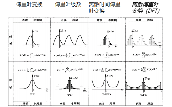
Symmetry law of signal in time and frequency domain (Fourier series, Fourier transform, discrete-time Fourier transform and discrete Fourier Series):

• Time domain periodic continuous → frequency domain discrete aperiodic (Fourier series FS)
• Time domain aperiodic continuous → frequency domain aperiodic continuous (Fourier transform FT)
• Aperiodic discrete in time domain → continuous periodic in frequency domain (discrete time Fourier transform DTFT)
• Discrete period in time domain → discrete period in frequency domain (Discrete Fourier series DFS)

9. Actual combat

Given a piece of audio, please extract 12 dimensional MFCC features and 23 dimensional FBank. The library you need to rely on is librosa.
Librosa is a python toolkit for audio and music analysis and processing. It has all the functions of common time-frequency processing, feature extraction, drawing sound graphics and so on.

#!/usr/bin/env python
# -*- coding:utf-8 -*-
# @FileName  :MFCC_test.py
# @Time      :2022/2/16 12:10
# @Author    :PangXZ
import librosa
import numpy as np
from scipy.fftpack import dct

# Draw spectrogram pictures
import matplotlib

matplotlib.use('Agg')
import matplotlib.pyplot as plt


def plot_spectrogram(spec, note, file_name):
    """
    Draw the spectrogram picture
    :param spec: a feature_dim by num_frames array (data)
    :param note: title of the picture
    :param file_name: name of the file
    :return:
    """
    fig = plt.figure(figsize=(20, 5))
    heatmap = plt.pcolor(spec)
    fig.colorbar(mappable=heatmap)
    plt.xlabel('Time(s')
    plt.ylabel(note)
    plt.tight_layout()
    plt.savefig(file_name)


def preemphasis(signal, coeff=0.97):
    """
    Speech signal pre emphasis is equivalent to a first-order high pass filter
    :param signal: speech signal 
    :param coeff:  Pre weighting coefficient,0 Indicates no emphasis. The default value is 0.97
    :return: Return the accented voice signal
    """
    return np.append(signal[0], signal[1:] - coeff * signal[:-1])


def enframe(signal, frame_len=400, frame_shift=160, win=np.hamming(M=400)):
    """
    Frame and windowing the voice signal (Hamming window)
    :param signal:      Input voice signal
    :param frame_len:   Frame length, where the number of sampling points in a frame is used
    :param frame_shift: Frame shift
    :param win:         Window type
    :return:            Return the voice signal after windowing
    """
    num_samples = signal.size  # Size of voice signal
    num_frames = np.floor((num_samples - frame_len) / frame_shift) + 1  # Number of frames
    frames = np.zeros((int(num_frames), frame_len))
    for i in range(int(num_frames)):
        frames[i, :] = signal[i * frame_shift: i * frame_shift + frame_len]
        frames[i, :] = frames[i, :] * win
    return frames


def get_spectrum(frames, fft_len=512):
    """
    The spectrum of speech signal is obtained by fast Fourier transform
    :param frames: Framing speech signal, num_frames by frame_len array
    :param fft_len:The length of fast Fourier transform is 512 by default
    :return: Return to the spectrum, a num_frames by fft_len/2+1 array (real)
    """
    cFFT = np.fft.fft(frames, n=fft_len)
    valid_len = int(fft_len / 2) + 1
    spectrum = np.abs(cFFT[:, 0:valid_len])
    return spectrum


def fbank(spectrum, num_filter=23, fft_len=512, sample_size=16000):
    """
    From the spectrum mel Filter bank characteristics
    :param spectrum:    spectrum
    :param num_filter:  mel The number of filters is 23 by default
    :return: return fbank features
    """
    # 1. Obtain a set of Mel filter banks
    low_freq_mel = 0
    high_freq_mel = 2595 * np.log10(1 + (sample_size / 2) / 700)  # Convert to mel scale
    mel_points = np.linspace(low_freq_mel, high_freq_mel, num_filter + 2)  # Linear point taking in mel space
    hz_points = 700 * (np.power(10., (mel_points / 2595)) - 1)  # Reversal linear spectrum
    bin = np.floor(hz_points / (sample_size / 2) * (fft_len / 2 + 1))  # Scale the original frequency corresponding value to the FFT window length
    # 2. Filter the feature of each frame with a filter bank, calculate the product of the feature and the filter, and use NP dot
    fbank = np.zeros((num_filter, int(np.floor(fft_len / 2 + 1))))
    for m in range(1, 1 + num_filter):
        f_left = int(bin[m - 1])    # Left boundary point
        f_center = int(bin[m])      # Center point
        f_right = int(bin[m + 1])   # Right boundary point
        for k in range(f_left, f_center):
            fbank[m - 1, k] = (k - f_left) / (f_center - f_left)
        for k in range(f_center, f_right):
            fbank[m - 1, k] = (f_right - k) / (f_right - f_center)
    filter_banks = np.dot(spectrum, fbank.T)
    # finfo function obtains information according to the type in parentheses and obtains the number type that conforms to this type
    # eps is the minimum non negative value, NP finfo(float). The value of eps is 2.220446049250313e-16, which is the smallest positive number
    filter_banks = np.where(filter_banks == 0, np.finfo(float).eps, filter_banks)
    # 3. Logarithmic operation
    filter_banks = 20 * np.log10(filter_banks)
    return filter_banks


def mfcc(fbank, num_mfcc=22):
    """
    be based on Fbank Feature acquisition MFCC features
    :param fbank:   fbank features
    :param num_mfcc: MFCC Number of coefficients
    :return: MFCC features
    """
    # feats = np.zeros((fbank.shape[0], num_mfcc))
    # 1. From the fbank feature obtained in the previous step, calculate the obtained mfcc feature, which is mainly a discrete cosine transform operation
    mfcc = dct(fbank, type=2, axis=1, norm='ortho')[:, 1:(num_mfcc + 1)]
    return mfcc


def write_file(feats, file_name):
    """
    Save feature to file
    :param feats:   Speech signal characteristics
    :param file_name: File name
    """
    f = open(file_name, 'w')
    (row, col) = feats.shape
    for i in range(row):
        f.write('[')
        for j in range(col):
            f.write(str(feats[i, j]) + ' ')
        f.write(']\n')
    f.close()


if __name__ == "__main__":
    # Pre weighting coefficient 0.97
    alpha = 0.97
    # Frame setting
    sample_size = 16000  # fs 16kHz
    frame_len = 400  # There are 400 sampling points in a frame, i.e. 16000 ×  0.025 = 400, sampling rate fs=16kHz, frame length 25ms
    frame_shift = 160  # Frame shift 10ms ×  Sampling rate 16kHz = 160
    fft_len = 512  # The sampling signal length of fast Fourier transform is 512 = the 9th power of 2

    # Mel filter bank settings
    num_filter = 23  # Number of filters
    num_mfcc = 12  # Number of cepstrums

    # Read WAV format voice file
    wav, fs = librosa.load('test.wav', sr=None)
    signal = preemphasis(wav, coeff=alpha)
    frames = enframe(signal, frame_len=frame_len, frame_shift=frame_shift, win=np.hamming(M=frame_len))
    spectrum = get_spectrum(frames, fft_len=fft_len)
    fbank_feats = fbank(spectrum, num_filter=num_filter, fft_len=fft_len, sample_size=sample_size)
    mfcc_feats = mfcc(fbank_feats, num_mfcc=num_mfcc)
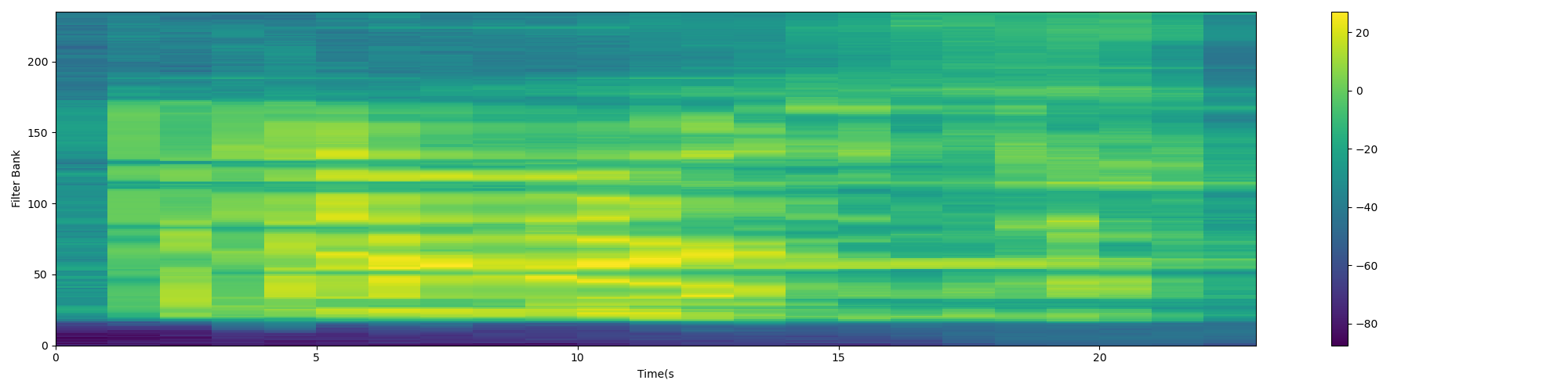
    plot_spectrogram(fbank_feats, 'Filter Bank', 'fbank.png')
    write_file(fbank_feats, 'test.fbank')
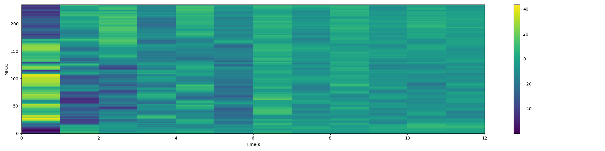
    plot_spectrogram(mfcc_feats, 'MFCC', 'mfcc.png')
    write_file(mfcc_feats, 'test.mfcc')

FBank spectrum diagram is as follows:

MFCC characteristic diagram:

reference material

1. Speech recognition: Principles and Applications
2. wave - read / write WAV format file
3. Instructions for using python standard library wave
4. contextlib: utility for creating and using context manager
5. Introduction to Fbank and MFCC - theory and code
6. How to understand that Fourier transform time domain continuous corresponds to frequency domain aperiodic, and time domain discrete corresponds to frequency domain periodic?
7. Discrete time Fourier transform (DTFT)
8. Symmetry law of signal in time and frequency domain