The most obvious feature that SQL differs FROM other programming languages is the order in which the code is processed. In large number programming languages, code is processed in coding order, but in SQL language, the first clause to be processed is the FROM clause. Although the SELECT statement appears first, it is almost always processed last.

Each step produces a virtual table that is used as input to the next step. These virtual tables are not available to callers (client applications or external queries). Only the tables generated in the last step will be returned to callers. If a clause is not specified in the query, the corresponding step will be skipped.

Let's start with a piece of pseudo code. Can you understand it first?

SELECT DISTINCT <select_list>
FROM <left_table>
<join_type> JOIN <right_table>
ON <join_condition>
WHERE <where_condition>
GROUP BY <group_by_list>
HAVING <having_condition>
ORDER BY <order_by_condition>
LIMIT <limit_number>

If you know the meaning and function of each keyword, it would be great if you have used it. However, do you know these statements and their execution order?

preparation

First of all, all test operations are completed on the MySQL database. For some simple operations on the MySQL database, please read the following article:

• <MySQL literacy>
• <Introduction to MySQL storage engine>
• <MySQL data types and properties>
• <MySQL common commands for dealing with databases and tables>

Continue to make the following preliminary preparations:

1. Create a new test database TestDB;

 create database TestDB;

2. Create test tables table1 and table2;

CREATE TABLE table1
 (
     customer_id VARCHAR(10) NOT NULL,
     city VARCHAR(10) NOT NULL,
     PRIMARY KEY(customer_id)
 )ENGINE=INNODB DEFAULT CHARSET=UTF8;

 CREATE TABLE table2
 (
     order_id INT NOT NULL auto_increment,
     customer_id VARCHAR(10),
     PRIMARY KEY(order_id)
 )ENGINE=INNODB DEFAULT CHARSET=UTF8;

3. Insert test data;

 INSERT INTO table1(customer_id,city) VALUES('163','hangzhou');
 INSERT INTO table1(customer_id,city) VALUES('9you','shanghai');
 INSERT INTO table1(customer_id,city) VALUES('tx','hangzhou');
 INSERT INTO table1(customer_id,city) VALUES('baidu','hangzhou');

 INSERT INTO table2(customer_id) VALUES('163');
 INSERT INTO table2(customer_id) VALUES('163');
 INSERT INTO table2(customer_id) VALUES('9you');
 INSERT INTO table2(customer_id) VALUES('9you');
 INSERT INTO table2(customer_id) VALUES('9you');
 INSERT INTO table2(customer_id) VALUES('tx');
 INSERT INTO table2(customer_id) VALUES(NULL);

After the preparation, table1 and table2 should look like the following:

 mysql> select * from table1;
 +-------------+----------+
 | customer_id | city     |
 +-------------+----------+
 | 163         | hangzhou |
 | 9you        | shanghai |
 | baidu       | hangzhou |
 | tx          | hangzhou |
 +-------------+----------+
 4 rows in set (0.00 sec)

 mysql> select * from table2;
 +----------+-------------+
 | order_id | customer_id |
 +----------+-------------+
 |        1 | 163         |
 |        2 | 163         |
 |        3 | 9you        |
 |        4 | 9you        |
 |        5 | 9you        |
 |        6 | tx          |
 |        7 | NULL        |
 +----------+-------------+
 7 rows in set (0.00 sec)

4. Prepare SQL logical query test statement

SELECT a.customer_id, COUNT(b.order_id) as total_orders
 FROM table1 AS a
 LEFT JOIN table2 AS b
 ON a.customer_id = b.customer_id
 WHERE a.city = 'hangzhou'
 GROUP BY a.customer_id
 HAVING count(b.order_id) < 2
 ORDER BY total_orders DESC;

Use the above SQL query statement to obtain customers from Hangzhou with less than 2 orders.

SQL logical query statement execution order

Remember the long string of SQL logical query rules given above? So, which is executed first and which is executed later? Now, let me give the execution order of a query statement:

(7)     SELECT 
(8)     DISTINCT <select_list>
(1)     FROM <left_table>
(3)     <join_type> JOIN <right_table>
(2)     ON <join_condition>
(4)     WHERE <where_condition>
(5)     GROUP BY <group_by_list>
(6)     HAVING <having_condition>
(9)     ORDER BY <order_by_condition>
(10)    LIMIT <limit_number>

The execution sequence number is indicated in front of each statement, so how are the query statements executed?

Introduction to logical query processing phase

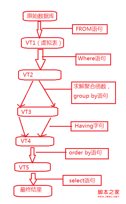
1. FROM: perform Cartesian product (cross join) on the first two tables in the FROM clause to generate virtual table VT1
2. ON: applies the ON filter to VT1. Only those that make < join_ The line whose condition > is true is inserted into VT2.
3. OUTER(JOIN): if OUTER JOIN (relative to CROSS JOIN or INNER JOIN) is specified, Retention table (preserved table: the left OUTER JOIN marks the left table as a reserved table, the right OUTER JOIN marks the right table as a reserved table, and the full OUTER JOIN marks both tables as reserved tables). If the FROM clause contains more than two tables, repeat step 1 for the result table generated by the previous join and the next table Go to step 3 until all tables are processed.
4. WHERE: apply WHERE filter to VT3. Only make < WHERE_ Only lines with condition > true are inserted into VT4
5. GROUP BY: group the rows in VT4 according to the column list in the GROUP BY clause to generate VT5
6. CUBE|ROLLUP: insert supergroups into VT5 to generate VT6
7. HAVING: applies the HAVING filter to VT6. Only make < HAVING_ Only groups with condition > true will be inserted into VT7
8. SELECT: process the SELECT list to generate VT8
9. DISTINCT: remove duplicate lines from VT8 to generate VT9
10. ORDER BY: sort the rows in VT9 according to the column list in the ORDER BY clause to generate a cursor (VC10)
11. TOP: select the specified number or proportion of rows from the beginning of VC10, generate table VT11, and return the caller.

Note:

Brief introduction to Cartesian product: assuming set A={a, b}, set B={0, 1, 2}, the Cartesian product of two sets is {(a, 0), (a, 1), (a, 2), (b, 0), (b, 1), (b, 2)}.

Step 10: sort the rows returned in the previous step according to the column list in the ORDER BY clause, and return the cursor VC10 This step is the first and only step to use the column alias in the SELECT list. Unlike other steps, this step does not return a valid table, but a cursor. SQL is based on set theory. A collection does not sort its rows in advance. It is just a logical collection of members, and the order of members does not matter. Queries that sort tables can return an object containing rows organized in a specific physical order. ANSI calls such objects cursors. Understanding this step is the basis for a correct understanding of SQL.

Because this step does not return to the table (instead of returning cursors), queries that use the ORDER BY clause cannot be used as table expressions. Table expressions include views, inline table valued functions, subqueries, derived tables, and common expressions. Its results must be returned to the client application that expects physical records. For example, the following derived table query is invalid and generates an error:

select * 
from(select orderid,customerid from orders order by orderid) 
as d

The following views also generate errors:

create view my_view
as
select *
from orders
order by orderid

In SQL, queries with an ORDER BY clause are not allowed in table expressions, but there is an exception in T-SQL (apply the TOP option).

So remember, don't assume any particular order for the rows in the table. In other words, do not specify the ORDER BY clause unless you are sure to order rows. Sorting requires cost.

#Execute FROM statement

During the execution of these SQL statements, a virtual table will be generated to save the execution results of SQL statements (this is the key point). Now I will track the changes of this virtual table and get the final query results to analyze the execution sequence and process of the whole SQL logical query.

The first step is to execute the FROM statement. We first need to know which table to start with, which is what FROM tells us. Now there is < left_ Table > and < right_ Table > which table do we start FROM, or do we start after some connection between the two tables? How do they connect—— Cartesian product

About what is Cartesian product, please help yourself. After performing Cartesian product on two tables through the FROM statement, you will get a virtual table, temporarily called VT1 (virtual table 1), as follows:

+-------------+----------+----------+-------------+
| customer_id | city     | order_id | customer_id |
+-------------+----------+----------+-------------+
| 163         | hangzhou |        1 | 163         |
| 9you        | shanghai |        1 | 163         |
| baidu       | hangzhou |        1 | 163         |
| tx          | hangzhou |        1 | 163         |
| 163         | hangzhou |        2 | 163         |
| 9you        | shanghai |        2 | 163         |
| baidu       | hangzhou |        2 | 163         |
| tx          | hangzhou |        2 | 163         |
| 163         | hangzhou |        3 | 9you        |
| 9you        | shanghai |        3 | 9you        |
| baidu       | hangzhou |        3 | 9you        |
| tx          | hangzhou |        3 | 9you        |
| 163         | hangzhou |        4 | 9you        |
| 9you        | shanghai |        4 | 9you        |
| baidu       | hangzhou |        4 | 9you        |
| tx          | hangzhou |        4 | 9you        |
| 163         | hangzhou |        5 | 9you        |
| 9you        | shanghai |        5 | 9you        |
| baidu       | hangzhou |        5 | 9you        |
| tx          | hangzhou |        5 | 9you        |
| 163         | hangzhou |        6 | tx          |
| 9you        | shanghai |        6 | tx          |
| baidu       | hangzhou |        6 | tx          |
| tx          | hangzhou |        6 | tx          |
| 163         | hangzhou |        7 | NULL        |
| 9you        | shanghai |        7 | NULL        |
| baidu       | hangzhou |        7 | NULL        |
| tx          | hangzhou |        7 | NULL        |
+-------------+----------+----------+-------------+

There are 28 records in total (number of records in table1 * number of records in table2). This is the result of VT1. The next operations are based on VT1.

#Perform ON filtering

After the Cartesian product is executed, proceed to ON a.customer_id = b.customer_id condition filtering: remove the data that does not meet the conditions according to the conditions specified in ON to obtain the VT2 table, which is as follows:

+-------------+----------+----------+-------------+
| customer_id | city     | order_id | customer_id |
+-------------+----------+----------+-------------+
| 163         | hangzhou |        1 | 163         |
| 163         | hangzhou |        2 | 163         |
| 9you        | shanghai |        3 | 9you        |
| 9you        | shanghai |        4 | 9you        |
| 9you        | shanghai |        5 | 9you        |
| tx          | hangzhou |        6 | tx          |
+-------------+----------+----------+-------------+

VT2 is the useful data obtained after ON condition filtering, and the next operations will continue ON the basis of VT2.

#Add external row

This step only occurs when the connection type is OUTER JOIN, such as LEFT OUTER JOIN, RIGHT OUTER JOIN and FULL OUTER JOIN. In most cases, we will omit the OUTER keyword, but OUTER represents the concept of external rows.

LEFT OUTER JOIN records the left table as a reserved table, and the result is:

+-------------+----------+----------+-------------+
| customer_id | city     | order_id | customer_id |
+-------------+----------+----------+-------------+
| 163         | hangzhou |        1 | 163         |
| 163         | hangzhou |        2 | 163         |
| 9you        | shanghai |        3 | 9you        |
| 9you        | shanghai |        4 | 9you        |
| 9you        | shanghai |        5 | 9you        |
| tx          | hangzhou |        6 | tx          |
| baidu       | hangzhou |     NULL | NULL        |
+-------------+----------+----------+-------------+

RIGHT OUTER JOIN records the right table as a reserved table, and the result is:

+-------------+----------+----------+-------------+
| customer_id | city     | order_id | customer_id |
+-------------+----------+----------+-------------+
| 163         | hangzhou |        1 | 163         |
| 163         | hangzhou |        2 | 163         |
| 9you        | shanghai |        3 | 9you        |
| 9you        | shanghai |        4 | 9you        |
| 9you        | shanghai |        5 | 9you        |
| tx          | hangzhou |        6 | tx          |
| NULL        | NULL     |        7 | NULL        |
+-------------+----------+----------+-------------+

FULL OUTER JOIN takes the left and right tables as reserved tables, and the results are as follows:

+-------------+----------+----------+-------------+
| customer_id | city     | order_id | customer_id |
+-------------+----------+----------+-------------+
| 163         | hangzhou |        1 | 163         |
| 163         | hangzhou |        2 | 163         |
| 9you        | shanghai |        3 | 9you        |
| 9you        | shanghai |        4 | 9you        |
| 9you        | shanghai |        5 | 9you        |
| tx          | hangzhou |        6 | tx          |
| baidu       | hangzhou |     NULL | NULL        |
| NULL        | NULL     |        7 | NULL        |
+-------------+----------+----------+-------------+

The work of adding external rows is to add the data filtered by the filter conditions in the reserved table on the basis of the VT2 table, give NULL values to the data in the non reserved table, and finally generate the virtual table VT3.

Since I used LEFT JOIN in the prepared test SQL query logic statement, the following data was filtered out:

| baidu       | hangzhou |     NULL | NULL        |

Now add this data to the VT2 table, and the VT3 table is as follows:

+-------------+----------+----------+-------------+
| customer_id | city     | order_id | customer_id |
+-------------+----------+----------+-------------+
| 163         | hangzhou |        1 | 163         |
| 163         | hangzhou |        2 | 163         |
| 9you        | shanghai |        3 | 9you        |
| 9you        | shanghai |        4 | 9you        |
| 9you        | shanghai |        5 | 9you        |
| tx          | hangzhou |        6 | tx          |
| baidu       | hangzhou |     NULL | NULL        |
+-------------+----------+----------+-------------+

The following operations will be performed on the VT3 table.

#Perform WHERE filtering

WHERE filtering is performed on the VT3 obtained by adding external rows, and only the VT3 that meets < WHERE_ Only the records of condition > will be output to virtual table VT4. When we execute WHERE a.city = 'hangzhou', we will get the following contents and store them in virtual table VT4:

+-------------+----------+----------+-------------+
| customer_id | city     | order_id | customer_id |
+-------------+----------+----------+-------------+
| 163         | hangzhou |        1 | 163         |
| 163         | hangzhou |        2 | 163         |
| tx          | hangzhou |        6 | tx          |
| baidu       | hangzhou |     NULL | NULL        |
+-------------+----------+----------+-------------+

However, when using the WHERE clause, you should pay attention to the following two points:

1. Because the data has not been grouped, you cannot use WHERE in the WHERE filter yet_ Condition = min (Col) filtering of grouping statistics;
2. Since the column has not been selected, it is not allowed to use the column alias in SELECT, such as: SELECT city as c FROM t WHERE c='shanghai '; Is not allowed.

#Execute GROUP BY grouping

The group by clause is mainly used to group the virtual tables obtained by using the WHERE clause. We execute group by a.customer in the test statement_ ID, you will get the following:

+-------------+----------+----------+-------------+
| customer_id | city     | order_id | customer_id |
+-------------+----------+----------+-------------+
| 163         | hangzhou |        1 | 163         |
| baidu       | hangzhou |     NULL | NULL        |
| tx          | hangzhou |        6 | tx          |
+-------------+----------+----------+-------------+

The obtained content will be stored in the virtual table VT5. At this time, we will get a VT5 virtual table, and the next operations will be completed on the table.

#Performing HAVING filtering

The HAVING clause is mainly used in conjunction with the GROUP BY clause to conditionally filter the VT5 virtual table obtained by grouping. When I execute HAVING count (b.order_id) < 2 in the test statement, I will get the following:

+-------------+----------+----------+-------------+
| customer_id | city     | order_id | customer_id |
+-------------+----------+----------+-------------+
| baidu       | hangzhou |     NULL | NULL        |
| tx          | hangzhou |        6 | tx          |
+-------------+----------+----------+-------------+

This is virtual table VT6.

#SELECT list

The SELECT clause will only be executed now. Don't think that the SELECT clause is written in the first line, which is the first to be executed.

We execute select a.customer in the test statement_ id, COUNT(b.order_id) as total_ Orders, select the content we need from the virtual table VT6. We will get the following:

+-------------+--------------+
| customer_id | total_orders |
+-------------+--------------+
| baidu       |            0 |
| tx          |            1 |
+-------------+--------------+

No, not yet. It's just virtual table VT7.

#Execute DISTINCT clause

If the DISTINCT clause is specified in the query, a temporary memory table will be created (if there is no memory, it needs to be stored on the hard disk). The table structure of this temporary table is the same as the virtual table VT7 generated in the previous step, except that a unique index is added to the column performing the DISTINCT operation to remove duplicate data.

Since DISTINCT is not used in my test SQL statement, this step will not generate a virtual table in this query.

#Execute ORDER BY clause

Sort the contents of the virtual table according to the specified column, and then return a new virtual table. We execute order by total in the test SQL statement_ Orders DESC, you will get the following:

+-------------+--------------+
| customer_id | total_orders |
+-------------+--------------+
| tx          |            1 |
| baidu       |            0 |
+-------------+--------------+

You can see that this is for total_ The orders column is arranged in descending order. The above results are stored in VT8.

Execute LIMIT clause

The LIMIT clause selects the specified row data starting from the specified position from the VT8 virtual table obtained in the previous step. For the LIMIT clause that does not apply ORDER BY, the results are also unordered. Therefore, many times, we will see that the LIMIT clause will be used together with the ORDER BY clause.

The MySQL database LIMIT supports the following options:

LIMIT n, m

Indicates that m records are selected from n records. Many developers like to use this statement to solve the paging problem. For small data, there is no problem using the LIMIT clause. When the amount of data is very large, using LIMIT n, m is very inefficient. Because the mechanism of LIMIT is to scan from the beginning every time. If you need to read three pieces of data from the 600000 line, you need to scan to 600000 lines first, and then read, and the scanning process is a very inefficient process. Therefore, for big data processing, it is very necessary to establish a certain caching mechanism in the application layer (it seems that all big data processing now have caching).

Reference documents:

SQL logical query statement execution sequence

Reproduced in https://www.cnblogs.com/Qian123/p/5669259.html