In this paper, Python statistical simulation method is used to introduce four commonly used statistical distributions, including discrete distribution: binomial distribution and Poisson distribution, and continuous distribution: exponential distribution and normal distribution. Finally, the distribution of height and weight data is checked.

# Import related modules
import pandas as pd
import numpy as np
import matplotlib.pyplot as plt
import seaborn as sns
%matplotlib inline
%config InlineBackend.figure_format = 'retina'

random number

After the invention of computer, a new way to solve the problem has come into being: using computer to simulate the real world. This method, also known as the Monte Carlo method, originated from the Manhattan Plan for the development of the atomic bomb in the United States during World War II. Among its inventors, von Neumann is well-known. The origin of the Monte Carlo method is also interesting. According to legend, the uncle of Ulam, another inventor, often loses money at Monte Carlo Casino in Morocco. Gambling is a game of probability, so the statistical simulation method based on probability is named after this casino.

Using statistical simulation, we first generate random numbers in Python. numpy.random The module provides a wealth of random number generating functions. For example, generate any random number between 0 and 1:

np.random.random(size=5)  # size denotes the number of generated random numbers

array([ 0.32392203,  0.3373342 ,  0.51677112,  0.28451491,  0.07627541])

Another example is to generate random integers in a certain range:

np.random.randint(1, 10, size=5)  # Generate five random integers between 1 and 9

array([5, 6, 9, 1, 7])

The random number generated by computer is actually pseudo-random number, which is calculated by a certain method. So we can specify the seeds generated by random number according to the following method. This advantage is that the same simulation results can be guaranteed when repeated calculation is carried out in the future.

np.random.seed(123)

In NumPy, not only the simple random numbers mentioned above can be generated, but also the corresponding random numbers can be generated according to a certain statistical distribution. Here we enumerate the corresponding random number generating functions of binomial distribution, Poisson distribution, exponential distribution and normal distribution. Next, we study the four types of statistical distribution.

• np.random.binomial()
• np.random.poisson()
• np.random.exponential()
• np.random.normal()

Binomial distribution

Binomial distribution It is the probability distribution of the number of times of success in n independent yes/no trials, in which the probability of success in each trial is p. This is a discrete distribution, so the probability mass function (PMF) is used to represent the probability of k times success.

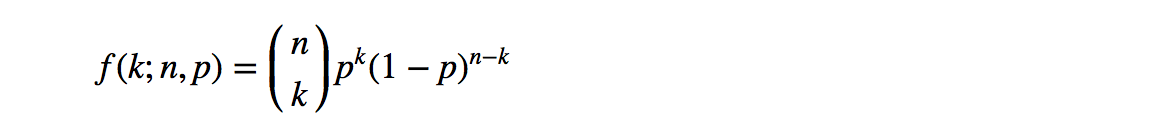
The most common binomial distribution is coin-tossing. If you toss n coins, the number of frontal upwards will satisfy the distribution. Next, we use computer simulation method to generate 10,000 binomial distribution random numbers, which correspond to 10,000 experiments. Each experiment throws n coins, and the number of coins facing up is the random number generated. At the same time, the PMF diagram of binomial distribution is drawn by using histogram function.

def plot_binomial(n,p):
    '''Drawing Probabilistic Mass Function of Binomial Distribution'''
    sample = np.random.binomial(n,p,size=10000)  # Generating 10,000 random numbers in binomial distribution
    bins = np.arange(n+2) 
    plt.hist(sample, bins=bins, align='left', normed=True, rwidth=0.1)  # Drawing Histogram
    #Setting titles and coordinates
    plt.title('Binomial PMF with n={}, p={}'.format(n,p))  
    plt.xlabel('number of successes')
    plt.ylabel('probability')


plot_binomial(10, 0.5)

If 10 coins are thrown with the same probability, i.e. p=0.5, the distribution of the number of positive coins coins coincides with the binomial distribution shown in the figure above. The distribution is symmetrical left and right, and the most likely case is that it occurs five times in the front.

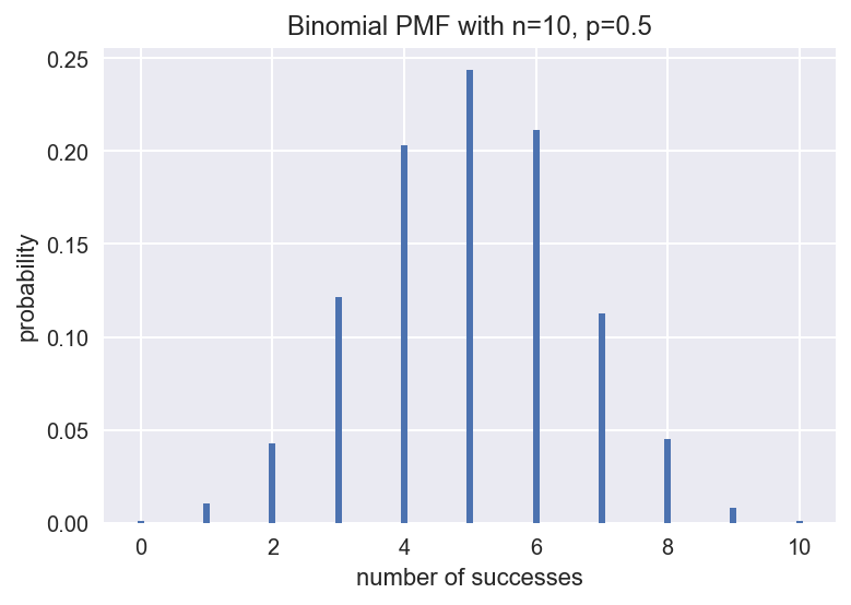
But what if it was a counterfeit coin? For example, what happens if the probability of facing up is p=0.2, or p=0.8? We can still draw the PMF diagram in this case.

fig = plt.figure(figsize=(12,4.5)) #settlngcanvassIze
p1 = fig.add_subplot(121)  # Add the first subgraph
plot_binomial(10, 0.2)
p2 = fig.add_subplot(122)  # Add a second subgraph
plot_binomial(10, 0.8)

At this point, the distribution is no longer symmetrical, as we expected, when the probability p=0.2, the front is most likely to occur twice, and when p=0.8, the front is most likely to occur eight times.

Poisson distribution

Poisson distribution It is used to describe the probability distribution of the number of random events per unit time. It is also a discrete distribution. Its probabilistic mass function is as follows:

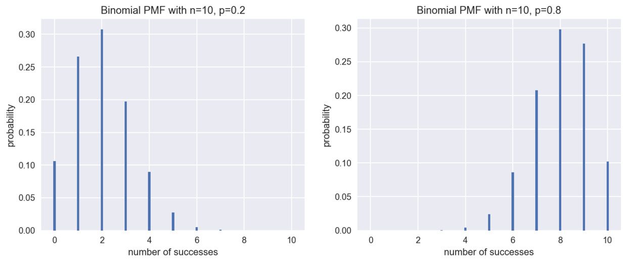
For example, if you are waiting for a bus, assuming that the arrival of these buses is independent and random (which is not realistic), there is no relationship between the front and rear buses, then the number of buses arriving in an hour conforms to the Poisson distribution. Similarly, the Poisson distribution is plotted by statistical simulation, assuming an average of six vehicles per hour (i.e., lambda=6 in the above formula).

lamb = 6
sample = np.random.poisson(lamb, size=10000)  # Generating 10,000 random numbers in accordance with Poisson distribution
bins = np.arange(20)
plt.hist(sample, bins=bins, align='left', rwidth=0.1, normed=True) # Drawing Histogram
# Setting headings and coordinate axes
plt.title('Poisson PMF (lambda=6)')
plt.xlabel('number of arrivals')
plt.ylabel('probability')
plt.show()

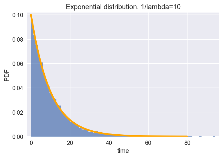
exponential distribution

exponential distribution It is used to describe the time interval of independent random events, which is a continuous distribution, so it is expressed by the mass density function.

For example, in the case of waiting for a bus, the time interval between the arrival of two cars conforms to the exponential distribution. Assuming that the average interval is 10 minutes (i.e. 1/lambda=10), your waiting time will satisfy the exponential distribution shown in the figure below from the last departure.

tau = 10
sample = np.random.exponential(tau, size=10000)  # Generating 10,000 random numbers satisfying exponential distribution
plt.hist(sample, bins=80, alpha=0.7, normed=True) #Drawing Histogram
plt.margins(0.02) 

# Drawing probability density function of exponential distribution according to formula
lam = 1 / tau
x = np.arange(0,80,0.1)
y = lam * np.exp(- lam * x)
plt.plot(x,y,color='orange', lw=3)

#Setting headings and coordinate axes
plt.title('Exponential distribution, 1/lambda=10')
plt.xlabel('time')
plt.ylabel('PDF')
plt.show()

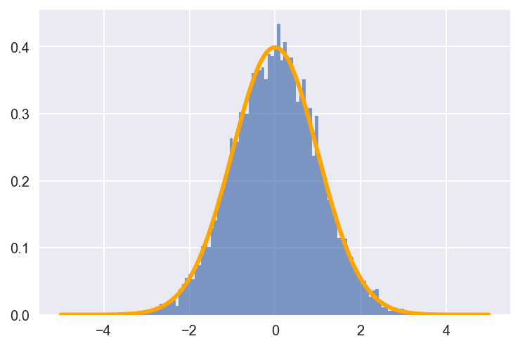
Normal distribution

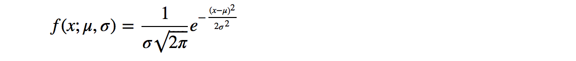
Normal distribution It is a very common statistical distribution, which can describe many things in the real world. It has very beautiful properties. We will introduce in detail the central limit theorem of parameter estimation in the next lecture. Its probability density function is:

The probability density curve of the normal distribution with the mean value of 0 and the standard deviation of 1 is plotted below. Its shape resembles a bell with an inverted mouth, so it is also called a bell curve.

def norm_pdf(x,mu,sigma):
    '''Normal distribution probability density function'''
    pdf = np.exp(-((x - mu)**2) / (2* sigma**2)) / (sigma * np.sqrt(2*np.pi))
    return pdf

mu = 0    # The mean is 0.
sigma = 1 # The standard deviation is 1.

# Drawing Histogram of Normal Distribution by Statistical Simulation
sample = np.random.normal(mu, sigma, size=10000)
plt. hist(sample, bins=100, alpha=0.7, normed=True)

# Drawing PDF Curve Based on Normal Distribution Formula
x = np.arange(-5, 5, 0.01)
y = norm_pdf(x, mu, sigma)
plt.plot(x,y, color='orange', lw=3)
plt.show()

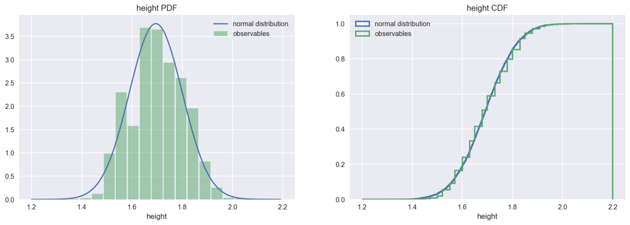
Distribution of height and weight

From the point of view of computer simulation, four kinds of distribution are introduced. Now let's look at the real data distribution. Continue with the previous lecture. Descriptive Statistics of Data Exploration Using the BRFSS data set, we look at the height and weight data to see if they meet the normal distribution.

Firstly, the data is imported, and plot_pdf_cdf() is written to draw PDF and CDF diagrams, which is easy to reuse.

# Import BRFSS data
import brfss
df = brfss.ReadBrfss()
height = df.height.dropna()
weight = df.weight.dropna()

def plot_pdf_cdf(data, xbins, xrange, xlabel):
    '''Drawing probability density function PDF Sum cumulative distribution function CDF'''

    fig = plt.figure(figsize=(16,5)) # Setting Canvas Size

    p1 = fig.add_subplot(121)  # Add the first subgraph
    # Drawing PDF Curve of Normal Distribution
    std = data.std()
    mean = data.mean()
    x = np.arange(xrange[0], xrange[1], (xrange[1]-xrange[0])/100)
    y = norm_pdf(x, mean, std)
    plt.plot(x,y, label='normal distribution')
    # Drawing Histogram of Data
    plt.hist(data, bins=xbins, range=xrange, rwidth=0.9, 
             alpha=0.5, normed=True, label='observables')
    # Picture Settings
    plt.legend()
    plt.xlabel(xlabel)
    plt.title(xlabel +' PDF')

    p2 = fig.add_subplot(122)  #Add a second subgraph
    # Drawing CDF Curve of Normal Distribution
    sample = np.random.normal(mean, std, size=10000)
    plt.hist(sample, cumulative=True, bins=1000, range=xrange, 
             normed=True, histtype='step', lw=2, label='normal distribution')
    # Drawing CDF Curves of Data
    plt.hist(data, cumulative=True, bins=1000, range=xrange, 
             normed=True, histtype='step', lw=2, label='observables')
    #Picture Settings
    plt.legend(loc='upper left')
    plt.xlabel(xlabel)
    plt.title( xlabel + ' CDF')
    plt.show()

The height distribution of the population accords with the normal distribution.

plot_pdf_cdf(data=height, xbins=21, xrange=(1.2, 2.2), xlabel='height')

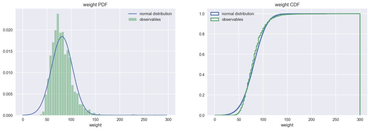
However, the body weight distribution is obviously right-sided, which is different from the symmetrical normal distribution.

plot_pdf_cdf(data=weight, xbins=60, xrange=(0,300), xlabel='weight')

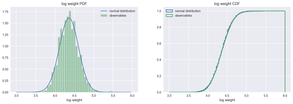
When the weight data are logarithmic, the distribution is in good agreement with the normal distribution.

log_weight = np.log(weight)
plot_pdf_cdf(data=log_weight, xbins=53, xrange=(3,6), xlabel='log weight')

This article code github

Data Exploration Series Catalogue:

1. Opening: Data Analysis Process
2. Descriptive statistics
3. Statistical Distribution (in this paper)
4. Estimation of parameters (to be continued)
5. Hypothesis testing (to be continued)

Reference material:

• Wikipedia: Monte Carlo Method
• <Think Stats 2>
• Statistics William Mendenhall

Thank:
Finally, I would like to thank the small partners of the big data community for their support and encouragement, so that we can grow together.