preface

I've been reading Dr. Li Hang's "statistical learning methods" recently. I'll make a small record here and write down my understanding. I welcome your criticism and correction.

text
Intuitive understanding of perceptron
Perceptron should be the simplest algorithm among machine learning algorithms. Its principle can be seen in the following figure: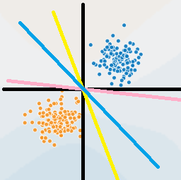
For example, we have a coordinate axis (black line in the figure), the horizontal axis is X1 and the vertical axis is x2. Every point in the figure is composed of (x1, x2). If we apply this diagram to judge whether the part is qualified, X1 represents the part length, X2 represents the part quality, the coordinate axis represents the average length and average weight of the part, and the blue is qualified product and the yellow is inferior product, which needs to be removed. Obviously, if the length and weight of the part are greater than the average, it indicates that the part is qualified Grid. That is, all the blue dots in the first quadrant. On the contrary, if both items are less than the mean, they are inferior, such as the yellow dot in the third quadrant.
But how do we make computers this rule?
The data set we know at present is the information and labels of all points in the current graph, that is, the amount of all samples (x1, x2). For these points above, it would be good if we could find a reasonable straight line to perfectly separate them. In this way, we can take a new sample and know its two parameters to judge its online side

We can see that we have many lines to separate the two points in the graph, but how to find the optimal dividing line?
In fact, our sensor can't find the best straight line. It may find the left and right lines drawn in the figure, but as long as all points can be separated.
Therefore: if a straight line can not be divided by one point, it is a good straight line.

Now let's talk about how to find this straight line? This line is first of all a line that can be divided into error classes of finite degrees. Therefore, we can calculate the sum of the distance between all the wrong points and the straight line, so that the minimum distance is the straight line we want to solve.
Mathematical formulas involved in perceptron
Because we do it in two categories, it is best to divide it into one positive and one negative. At that time, we design a + 1 and a - 1, which can be perfectly divided into two categories.
So we get a function: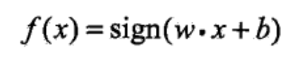
The specific definition of this sign function is as follows:

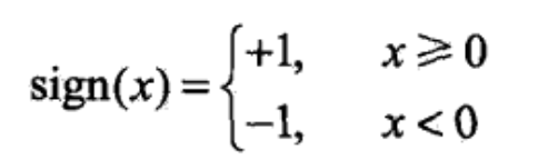
When the independent variable x is not less than 0, the function value is positive 1. When the independent variable x is less than 0, the function value is - 1
So, what is wx+b we introduced above?
It is the best straight line. Let's look at this formula in two dimensions. The straight line in two dimensions is defined as follows: y=ax+b. In two dimensions, w is a, b or b. So wx+b is a straight line (for example, the blue line in the figure at the beginning of this article). If the new point x is on the left of the blue line, then wx+b < 0, then it passes through sign, and finally f outputs - 1. If it is on the right, it outputs 1. Etc., it seems a little unreasonable. The situation is equivalent to a two-dimensional plane, y=ax+b. as long as the point is above the X axis, regardless of the left and right sides of the point line, the final result is greater than 0. This value is positive or negative What does it have to do with the line? emmm... In fact, wx+b and ax+b express the same form of a straight line, but they are slightly different. Let's rotate the top picture 45 degrees counterclockwise. Does the blue line become the X axis? Haha, is the right side of the original blue line above the X axis? In fact, when the perceptron calculates the line wx+b, it has been secretly converted, so that the straight line used for division becomes the x-axis, and the left and right sides are above and below the x-axis respectively, which becomes positive and negative.
So what's the difference between wx+b and ax+b?
In this paper, parts are used as an example, The length and weight (x1, x2) are used to represent the attributes of a part, so a two-dimensional plane is sufficient. If the quality of the part is also related to the color, then a X3 must be added to represent the color, and the attributes of the sample become (x1, X2, x3) becomes three-dimensional. wx+b is not only used in two-dimensional cases, but can still be used in three-dimensional cases. Therefore, wx+b and ax+b are only approximately the same in two-dimensional, which is actually different. What is wx+b in three-dimensional? If we imagine that there are blue dots in one corner, yellow dots in one corner and a straight line in one corner of the room, it is obviously not Enough, need a plane! So in three dimensions, wx+b is a plane! As for why, it will be explained in detail later. What about the fourth dimension? emmm... It seems impossible to describe what can separate the four-dimensional space, but for the four-dimensional space, there should be something that cuts the four-dimensional space in half like a knife. If it can be cut in half, it should be a plane for four dimensions, just as for three dimensions, it is a two-dimensional plane, and two dimensions are a one-dimensional plane. In short, wx+b in four dimensions can be expressed as something that is a plane relative to four dimensions, and then divide all four-dimensional space into two. We call it hyperplane. Thus, in high-dimensional space, wx+b is a partitioned hyperplane, which is its formal name.
Generally speaking, wx+b corresponds to the hyperplane S in n-dimensional space, where w is the normal vector of the hyperplane and b is the intercept of the hyperplane. This hyperplane divides space into two parts. Points in two parts are divided into positive and negative, so hyperplane S is also called separated hyperplane.

How to calculate the distance

From the initial requirement of having an f(x), we can only output 1 and - 1 sign(x), and then to the current wx+b, it seems more and more simple. As long as we can find the most appropriate wx+b, we can complete the construction of the perceptron. As mentioned earlier, to find this hyperplane by maximizing the distance between misclassified points, first we need to give a formula to calculate the distance between a point and the hyperplane separately, as follows: hi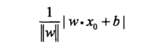
In two-dimensional space, we can think of it as a straight line, but after the transformation, wx+b is the x-axis after the whole graph is rotated, and the distance from all points to the x-axis is actually the absolute value of wx+b. Then we find the sum of the distances of all misclassification points, that is, the sum of | wx+b | to minimize it. When we compare numerical values, it is more convenient to calculate with smaller values. Therefore, we need to reduce the overall value by n times, but how much is it? Our experience tells us that the unit length is the best comparison, so we can divide by | w |, so we can get the above form.
Definition of loss function

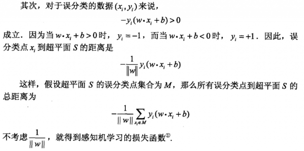
For misclassified data, such as points that should actually belong to the positive category, but actually predicted to be the negative category. For the wrong category, we should add a minus sign at this time, and the result is positive.
|wx+b | is called the function interval, and it is called the geometric interval after dividing the module length. The geometric interval can be regarded as the actual length in the physical sense. No matter how you zoom in or out, your physical distance is like that. It is impossible to change the number. When calculating the distance in machine learning, geometric interval is usually used, otherwise the solution cannot be obtained.
But the above says that it becomes a function interval without considering dividing by the module length. Why can we do this?
An explanation is given below: the perceptron is a misclassification driven algorithm, and its ultimate goal is to have no misclassification points. If there are no misclassification points, the total distance becomes 0, and the values of w and b are useless. Therefore, there is no difference between geometric interval and function interval in the application of perceptron. In order to simplify the calculation, function interval is used.

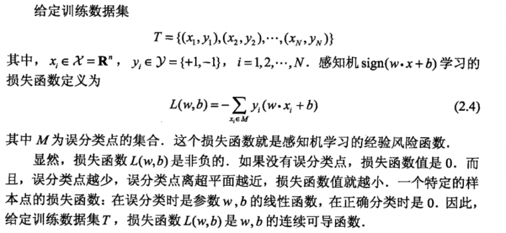
The above is the formal definition of loss function. The ultimate goal in finding the partition hyperplane is to minimize the loss function. If it is 0, it is of course the best.

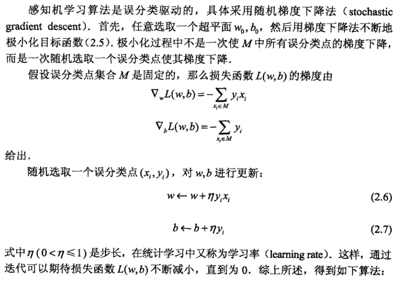
The perceptron uses the gradient descent method to obtain the optimal solutions of w and b, so as to obtain the partition hyperplane wx+b.
(gradient descent algorithm will be sorted out later)
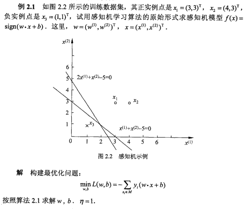
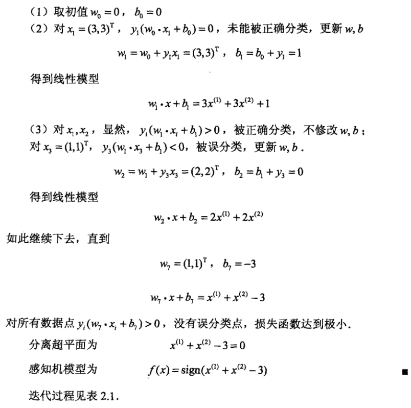
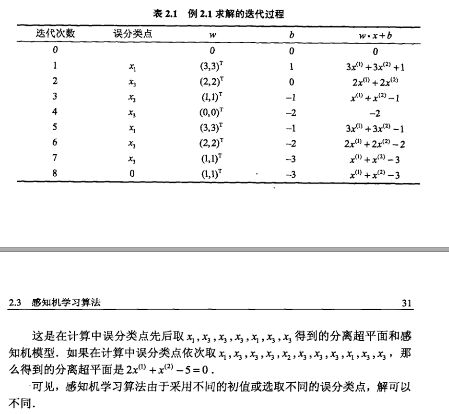
The following example is the example in Dr. Li Hang's statistical learning methods:

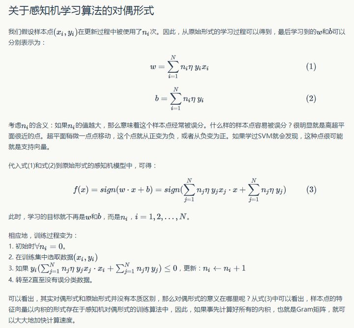
Dual form of perceptron learning

The specific process is as follows:

Implementation code:

#coding=utf-8
#Author:Dodo
#Date:2018-11-15
#Email:lvtengchao@pku.edu.cn

'''
Dataset: Mnist
 Number of training sets: 60000
 Number of test sets: 10000
------------------------------
Operation results:
Accuracy: 81.72%((II) classification
 Run time: 78.6s
'''

import numpy as np
import time

def loadData(fileName):
    '''
    load Mnist data set
    :param fileName:The path of the dataset to load
    :return: list Formal data sets and Tags
    '''
    print('start to read data')
    # list for storing data and marks
    dataArr = []; labelArr = []
    # Open file
    fr = open(fileName, 'r')
    # Read files by line
    for line in fr.readlines():
        # Cut each row of data by ',' and return to the field list
        curLine = line.strip().split(',')

        # Mnsit has 0-9 marks. Since it is a secondary classification task, it takes > = 5 as 1 and < 5 as - 1
        if int(curLine[0]) >= 5:
            labelArr.append(1)
        else:
            labelArr.append(-1)
        #Storage mark
        #[int (Num) for num in curline [1:]] - > traverse each line and convert all elements into int type except the first brother element (tag)
        #[int (Num) / 255 for num in curline [1:]] - > normalize all data except 255 (it is not a necessary step and can not be normalized)
        dataArr.append([int(num)/255 for num in curLine[1:]])

    #Return data and label
    return dataArr, labelArr

def perceptron(dataArr, labelArr, iter=50):
    '''
    Perceptron training process
    :param dataArr:Training set data (list)
    :param labelArr: Label of training set(list)
    :param iter: Number of iterations, 50 by default
    :return: Trained w and b
    '''
    print('start to trans')
    #Convert data into matrix form (in machine learning, because it is usually vector operation, conversion is called matrix form for convenient operation)
    #The vector of each sample in the converted data is horizontal
    dataMat = np.mat(dataArr)
    #Convert the label into a matrix and transpose it (. T is transpose).
    #Transpose is because an element in the label needs to be taken separately in the operation. If it is a 1xN matrix, it cannot be read in the way of label[i]
    #For a label with only 1xN, you can directly label[i] without converting it into a matrix. The conversion here is for the unification of format
    labelMat = np.mat(labelArr).T
    #Gets the size of the data matrix, m*n
    m, n = np.shape(dataMat)
    #Create the initial weight w, and the initial values are all 0.
    #np. The return value of shape (datamat) is m, N - > NP The value of shape (datamat) [1]) is n, and
    #The sample length is consistent
    w = np.zeros((1, np.shape(dataMat)[1]))
    #Initialization offset b is 0
    b = 0
    #The initialization step, that is, n in the gradient descent process, controls the gradient descent rate
    h = 0.0001

    #Iterate the iter times
    for k in range(iter):
        #Gradient descent is performed for each sample
        #In Li Hang's book, in 2.3 1 the gradient descent used in the beginning part is unified after all samples are calculated
        #Perform a gradient descent
        #In 2.3 It can be seen in the second half of 1 (for example, formula 2.6 and 2.7). The summation symbol is gone. At this time, it is used
        #Is random gradient descent, that is, a gradient descent is performed for a sample after calculating a sample.
        #The differences between the two have their own advantages, but the more commonly used is random gradient descent.
        for i in range(m):
            #Gets the vector of the current sample
            xi = dataMat[i]
            #Get the label corresponding to the current sample
            yi = labelMat[i]
            #Determine whether it is a misclassification sample
            #The special diagnosis of misclassified samples is: - Yi (w * Xi + b) > = 0. For details, please refer to 2.2 in the book Subsection 2
            #The formula in the book says > 0. In fact, if = 0, it means that the change point is on the hyperplane, which is also incorrect
            if -1 * yi * (w * xi.T + b) >= 0:
                #For misclassified samples, gradient descent is performed to update w and b
                w = w + h *  yi * xi
                b = b + h * yi
        #Print training progress
        print('Round %d:%d training' % (k, iter))

    #Return to w and b after training
    return w, b


def model_test(dataArr, labelArr, w, b):
    '''
    Test accuracy
    :param dataArr:Test set
    :param labelArr: Test set label
    :param w: Weight gained from training w
    :param b: Training acquired bias b
    :return: Correct rate
    '''
    print('start to test')
    #Convert the data set into matrix form for convenient operation
    dataMat = np.mat(dataArr)
    #Convert the label into a matrix and transpose it. For details, refer to perceptron above
    #Explanation of this part
    labelMat = np.mat(labelArr).T

    #Gets the size of the test dataset matrix
    m, n = np.shape(dataMat)
    #Error sample count
    errorCnt = 0
    #Traverse all test samples
    for i in range(m):
        #Obtain a single sample vector
        xi = dataMat[i]
        #Obtain the sample tag
        yi = labelMat[i]
        #Obtain operation results
        result = -1 * yi * (w * xi.T + b)
        #If - Yi (w * Xi + b) > = 0, the sample is misclassified, and the number of wrong samples is increased by one
        if result >= 0: errorCnt += 1
    #Accuracy = 1 - (number of sample classification errors / total number of samples)
    accruRate = 1 - (errorCnt / m)
    #Return accuracy
    return accruRate

if __name__ == '__main__':

    #Get current time
    #The current time is also obtained at the end of the text. The difference between the two times is the program running time
    start = time.time()

    #Get training sets and Tags
    trainData, trainLabel = loadData('../Mnist/mnist_train.csv')
    #Get test sets and labels
    testData, testLabel = loadData('../Mnist/mnist_test.csv')

    #Training gain weight
    w, b = perceptron(trainData, trainLabel, iter = 30)
    #Test to obtain the correct rate
    accruRate = model_test(testData, testLabel, w, b)

    #Gets the current time as the end time
    end = time.time()
    #Display accuracy
    print('accuracy rate is:', accruRate)
    #Display duration
    print('time span:', end - start)

Reference links for this article: Add link description