1 Preface

Perceptron is a linear classification model of binary classification. Input: the feature vector of the instance; Output: the category of the instance [generally take the binary values of - 1 and + 1].

The perceptron corresponds to the separation hyperplane that divides the instance into positive and negative categories in the input space (feature space), which belongs to the discrimination model. Perceptron learning aims to find the hyperplane that linearly divides the training data. Therefore, the loss function based on misclassification is introduced, and the gradient descent method is used to minimize the loss function to find the perceptron model.

Perceptron is divided into primitive mode and dual form.

2 perceptron model

Definition 2.1 (perceptron) assumes that the input space (feature space) is χ ⊆ R n \chi \subseteq R^n χ ⊆ Rn, the input space is Y ⊆ { − 1 , + 1 } \mathcal{Y} \subseteq \left \{ -1,+1 \right \} Y ⊆ {− 1, + 1}, input x ∈ χ x\in \chi x∈ χ A feature vector representing an instance, corresponding to a point in the input space (feature space); input y ∈ Y y \in \mathcal{Y} Y ∈ Y represents the category of the instance. The following functions from input space to output space:
f ( x ) = s i g n ( w ⋅ x + b ) f(x)=sign(w\cdot x+b) f(x)=sign(w⋅x+b)
It's called a perceptron. Among them, w w w and b b b is the perceptron model parameter, w ∈ R n w\in R^n w ∈ Rn is called weight or weight vector, b ∈ R b \in R b ∈ R is called bias, w ⋅ x w\cdot x w ⋅ x is called w w w and b b Inner product of b. sign is a symbolic function, i.e
s i g n = {  +1  , x ≥ 0  -1  , x < 0 sign=\begin{cases} & \text{ +1 }, x\ge 0 \\ & \text{ -1 } ,x< 0 \end{cases} sign={​ +1 ,x≥0 -1 ,x<0​
Perceptron s i n g ( w ⋅ x ) sing(w\cdot x) The loss function of sing(w ⋅ x) learning is defined as
L ( w , b ) = − ∑ x i ∈ M y i ( w ⋅ x i + b ) L(w,b)=-\sum_{x_i\in M}^{} y_i(w\cdot x_i+b) L(w,b)=−xi​∈M∑​yi​(w⋅xi​+b)
among M M M is the set of misclassification points. This loss function is the empirical risk function of perceptron learning. L ( w , b ) L(w,b) L(w,b) is nonnegative.

3 original form of perceptron learning algorithm

Input:

Training data set T = { ( x 1 , y 1 ) ( x 2 , y 2 ) , ... , ( x N , y N ) } T = \left \{ \left ( x_1,y_1 \right ) \left ( x_2,y_2 \right ),\dots ,\left ( x_N,y_N \right ) \right \} T={(x1, y1) (x2, y2),..., (xN, yN)}, where x i ∈ X = R n x_i\in X=R^n xi​∈X=Rn， y i ∈ Y = − 1 , + 1 y_i\in Y={-1,+1} yi​∈Y=−1,+1， i = 1 , 2 , ... , N i=1,2,...,N i=1,2,…,N； Learning rate η ( 0 < η ≤ 1 ) η(0<η≤1) η(0<η≤1)；

Output:

w w w, b b b； Perceptron model f ( x ) = s i g n ( w ⋅ x + b ) f(x)=sign(w⋅x+b) f(x)=sign(w⋅x+b).

1. Select initial value w 0 , b 0 w_0,b_0 w0​,b0​；

2. Select data in training set ( x i , y i ) (x_i,y_i) (xi​,yi​)；

3. If y i ( w ⋅ x + b ) ≤ 0 y_i (w⋅x+b)≤0 yi​(w⋅x+b)≤0，
   w = w + η y i x i b = b + η y i w=w+ηy_i x_i\\ b=b+ηy_i w=w+ηyi​xi​b=b+ηyi​

   Turn to 2 until there are no misclassification points in the training set.

import numpy as np
# Data linearly separable
# Here is the univariate linear equation
class Model:
    def __init__(self, data):
        self.w = np.ones(len(data[0]) - 1, dtype=np.float32)
        self.b = 0
        self.eta = 0.1  # Learning rate
    # Random gradient descent method
    def fit(self, X_train, y_train):
        train_complete_flag = False
        while not train_complete_flag:
            wrong_count = 0
            for d in range(len(X_train)):
                X = X_train[d]
                y = y_train[d]
                if y * np.sign(np.dot(X, self.w) + self.b) <= 0:
                    self.w = self.w + self.eta * np.dot(y, X)
                    self.b = self.b + self.eta * y
                    wrong_count += 1
            if wrong_count == 0:
                train_complete_flag = True
        print("Training complete")
        print("weight w: ", self.w)
        print("bias b: ", self.b)

4 dual form of perceptron learning algorithm

Input:

Training data set T = { ( x 1 , y 1 ) ( x 2 , y 2 ) , ... , ( x N , y N ) } T = \left \{ \left ( x_1,y_1 \right ) \left ( x_2,y_2 \right ),\dots ,\left ( x_N,y_N \right ) \right \} T={(x1, y1) (x2, y2),..., (xN, yN)}, where x i ∈ X = R n x_i\in X=R^n xi​∈X=Rn， y i ∈ Y = − 1 , + 1 y_i\in Y={-1,+1} yi​∈Y=−1,+1， i = 1 , 2 , ... , N i=1,2,...,N i=1,2,…,N； Learning rate η ( 0 < η ≤ 1 ) η(0<η≤1) η(0<η≤1)；

Output:

α i , b α_i,b α i​,b； Perceptron model f ( x ) = s i g n ( ∑ j = 1 N α j y j x j ⋅ x + b ) f(x)=sign(\sum_{j=1}^{N} \alpha_j y_j x_j ⋅x+b) f(x)=sign(∑j=1N​ α J ⋅ yj ⋅ xj ⋅ x+b), where α = ( α 1 , α 2 , ... , α n ) T α=(α_1,α_2,...,α_n )^T α=(α1​,α2​,...,αn​)T.

1. α = 0 , b = 0 α=0,b=0 α=0,b=0；
2. Select data in training set ( x i , y i ) (x_i,y_i) (xi​,yi​)；
3. If y i ( ∑ j = 1 N α j y j x j ⋅ x + b ) ≤ 0 y_i(\sum_{j=1}^{N} \alpha_j y_j x_j ⋅x+b)≤0 yi​(∑j=1N​αj​yj​xj​⋅x+b)≤0，
   α i = α i + η b = b + η y i α_i=α_i+η\\ b=b+ηy_i αi​=αi​+ηb=b+ηyi​
   Go to 2 until there are no misclassification points in the training set.

In the dual form, the training examples only appear in the form of inner product. For convenience, the inner product between instances in the training set can be calculated in advance and stored in the form of a matrix, which is the so-called Gram matrix
G = [ x i ∙ y i ] N × N G=[x_i∙y_i ]_{N \times N} G=[xi​∙yi​]N×N​

# Dual form
import numpy as np
# Data linearly separable
# Here is the univariate linear equation
class Model:
    def __init__(self, X):
        self.alpha = np.zeros(X.shape[0])
        self.b = 0
        self.eta = 0.1  # Learning rate
        self.Gram = np.dot(X, X.T)  # Store Gram matrix multiplied by two

    # Random gradient descent method
    def fit(self, X_train, y_train):
        train_complete_flag = False
        while not train_complete_flag:
            wrong_count = 0
            for i in range(len(X_train)):
                X = X_train[i]
                y = y_train[i]
                # Update alpha when there is a point classification error_ I and paranoia
                tmp_sum = np.dot(np.multiply(self.alpha, y_train), self.Gram[:, i])
                # tmp_sum = 0
                # for j in range(X.shape[0]):
                #     tmp_sum += self.alpha[j] * y_train[j] * self.Gram[j, i]

                if y * (tmp_sum + self.b) <= 0:
                    self.alpha[i] += self.eta
                    self.b += self.eta * y
                    wrong_count += 1
            if wrong_count == 0:
                train_complete_flag = True
                # Calculate weights after training
                self.w = np.dot(np.multiply(self.alpha, y_train), X_train)

        print("Training complete")
        print("weight w: ", self.w)
        print("bias b: ", self.b)

5 built in functions

import matplotlib.pyplot as plt
import pandas as pd
import numpy as np
from sklearn.datasets import load_iris
import sklearn
from sklearn.linear_model import Perceptron

# load data
iris = load_iris()
df = pd.DataFrame(iris.data, columns=iris.feature_names)
df['label'] = iris.target
df.columns = [
    'sepal length', 'sepal width', 'petal length', 'petal width', 'label'
]
df.label.value_counts()

plt.figure()
plt.scatter(df[:50]['sepal length'], df[:50]['sepal width'], label='0')
plt.scatter(df[50:100]['sepal length'], df[50:100]['sepal width'], label='1')
plt.xlabel('sepal length')
plt.ylabel('sepal width')
plt.legend()

data = np.array(df.iloc[:100, [0, 1, -1]])
X, y = data[:, :-1], data[:, -1]
y = np.array([1 if i == 1 else -1 for i in y])

sklearn.__version__

clf = Perceptron(fit_intercept=True, max_iter=1000, shuffle=True)
clf.fit(X, y)

print("Weights assigned to the features: ", clf.coef_)
print("Constants in decision function:", clf.intercept_)

# canvas size 
plt.figure(figsize=(10, 10))

# Chinese title
plt.rcParams['font.sans-serif'] = ['SimHei']
plt.rcParams['axes.unicode_minus'] = False
plt.title('Iris linear data example')
plt.scatter(data[:50, 0], data[:50, 1], c='b', label='Tris-setosa')
plt.scatter(data[50:100, 0], data[50:100, 1], c='orange', label='Iris-versicolor')

# Draw the line of the sensor
x_points = np.arange(4, 8)
y_ = -(clf.coef_[0][0] * x_points + clf.intercept_) / clf.coef_[0][1]
plt.plot(x_points, y_)

# Other parts
plt.legend()
plt.grid(False)
plt.xlabel('sepal length')
plt.ylabel('sepal width')
plt.legend()
plt.show()

6 others

import pandas as pd
import numpy as np
from sklearn.datasets import load_iris  # Import yingweihua data
import matplotlib.pyplot as plt
import Perceptron_Dual
import Perceptron
from timeit import default_timer as timer

# Support Chinese
plt.rcParams['font.sans-serif'] = ['SimHei']  # Used to display Chinese labels normally
plt.rcParams['axes.unicode_minus'] = False  # Used to display negative signs normally

# load data
iris = load_iris()
df = pd.DataFrame(iris.data, columns=iris.feature_names)
df['label'] = iris.target

df.columns = [
    'sepal length', 'sepal width', 'petal length', 'petal width', 'label'
]
df.label.value_counts()
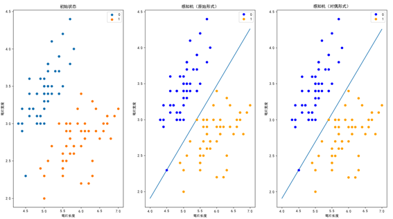
plt.subplot(1, 3, 1)
plt.scatter(df[:50]['sepal length'], df[:50]['sepal width'], label='0')
plt.scatter(df[50:100]['sepal length'], df[50:100]['sepal width'], label='1')
plt.xlabel('sepal length ')
plt.ylabel('sepal width ')
plt.title('Initial state')
plt.legend()

data = np.array(df.iloc[:100, [0, 1, -1]])
X, y = data[:, :-1], data[:, - 1]
y = np.array([1 if i == 1 else -1 for i in y])

'''
Original form
'''
tic = timer()
perceptron = Perceptron.Model(X)
perceptron.fit(X, y)

x_points = np.linspace(4, 7, 10)
y_ = -(perceptron.w[0] * x_points + perceptron.b) / perceptron.w[1]
plt.subplot(1, 3, 2)
plt.plot(x_points, y_)
plt.plot(data[:50, 0], data[:50, 1], 'bo', color='blue', label='0')
plt.plot(data[50:100, 0], data[50:100, 1], 'bo', color='orange', label='1')
plt.xlabel('sepal length ')
plt.ylabel('sepal width ')
plt.title('Perceptron (original form)')
plt.legend()
toc = timer()
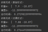
print("Run time:", toc - tic)

'''
Dual form
'''
tic = timer()
perceptron = Perceptron_Dual.Model(X)
perceptron.fit(X, y)

x_points = np.linspace(4, 7, 10)
y_ = -(perceptron.w[0] * x_points + perceptron.b) / perceptron.w[1]
plt.subplot(1, 3, 3)
plt.plot(x_points, y_)
plt.plot(data[:50, 0], data[:50, 1], 'bo', color='blue', label='0')
plt.plot(data[50:100, 0], data[50:100, 1], 'bo', color='orange', label='1')
plt.xlabel('sepal length ')
plt.ylabel('sepal width ')
plt.title('Perceptron (dual form)')
plt.legend()
toc = timer()
print("Run time:", toc - tic)
plt.show()

Operation results: