Reading guide

Time series prediction is a classical problem, which has been widely studied and applied in academia and industry. Even after adding the time dimension, everything in the world can be abstracted into time series problems, such as stock prices, weather changes and so on. The related theories of time series prediction are also very extensive. In addition to various classical statistical models, the current hot machine learning and cyclic neural network in deep learning can also be used for the modeling of time series prediction. Today, this paper will introduce the simple application of the three methods and verify them on a real time series data set.

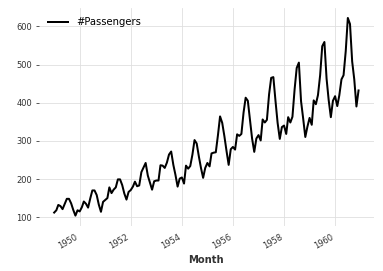
The main task of time series prediction is to predict its value in the future based on the historical data of a certain index. For example, the curve in the above figure records the monthly flight passengers in 144 months for 12 years from 1949 to 1960 (the specific unit has not been verified). Then the problem to be solved in time series prediction is: given the historical data of the previous 9 years, such as 1949-1957, So can we predict the number of passengers between 1958 and 1960.

In order to solve this problem, there are probably four mainstream solutions:

• Statistical model, the more classic ar series, including AR, MA, ARMA and ARIMA. In addition, the Prophet model launched by Facebook (to be exact, it should be called Meta now) is actually a statistical model. It is just a statistical model. On the basis of traditional trends and periodic components, it further refines and considers the influence of holidays, timing inflection points and other factors, In order to bring more accurate depiction of time sequence law;
• Machine learning model: in supervised machine learning, the regression problem mainly solves the problem of predicting the possible value of a Label based on a series of features. When taking historical data as features, it is natural to abstract the time series prediction problem into a regression problem. From this point of view, all regression models can be used to solve the time series prediction. For abstracting time series forecasting with machine learning, it is recommended to check the paper Machine Learning Strategies for Time Series Forecasting;
• Deep learning model, the mainstream application scenarios of deep learning belong to the two fields of CV and NLP, of which the latter is specially used to solve the problem of modeling sequence problems, and time series of course belongs to a special form of sequence data, so it is natural to use cyclic neural network to model time series prediction;
• Hidden Markov model, which is a classical abstraction used to describe the transition between adjacent states, and hidden Markov model further adds hidden states to enrich the expression ability of the model. However, one of the major assumptions is that the future state is only related to the current state, which is not conducive to using multiple historical states to jointly participate in the prediction. The more commonly used example may be weather prediction.

This paper mainly considers the first three time series prediction modeling methods, and selects: 1) Prophet model, 2) RandomForest regression model and 3) LSTM to test.

Firstly, the test is carried out on the real flight passenger data set, and the prediction accuracy of the three selected models is compared in turn. The data set includes the number of passengers per month in 12 years. January 1958 is used as the segmentation interface to divide the training set and test set, that is, the data of the first 9 years are used as the training set, and the data of the last 3 years are used as the test set to verify the effect of the model. The schematic diagram after data set segmentation is as follows:

df = pd.read_csv("AirPassengers.csv", parse_dates=["date"]).rename(columns={"date":"ds", "value":"y"})
X_train = df[df.ds<"19580101"]
X_test = df[df.ds>="19580101"]

plt.plot(X_train['ds'], X_train['y'])
plt.plot(X_test['ds'], X_test['y'])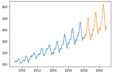

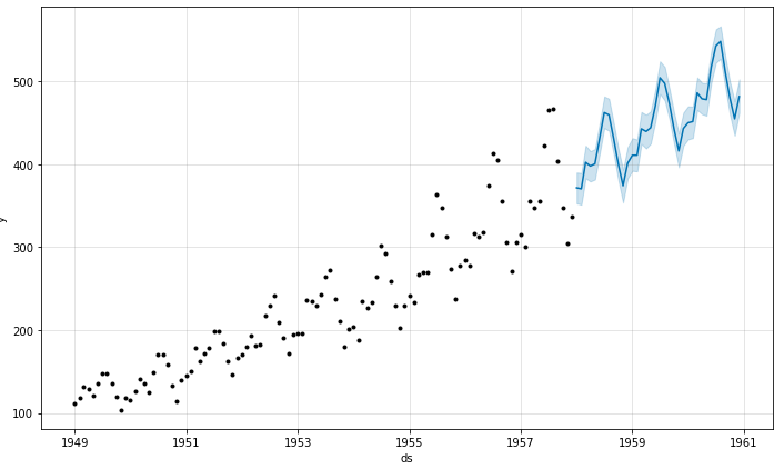
1. Prediction of Prophet model. Prophet is a highly encapsulated time series prediction model. It accepts a DataFrame as the training set (ds and y field columns are required). It also accepts a DataFrame during prediction, but only ds column is required at this time. For detailed introduction of the model, please refer to its official document: https://facebook.github.io/prophet/ . The core codes of model training and prediction are as follows:

from prophet import Prophet
pro = Prophet()
pro.fit(X_train)
pred = pro.predict(X_test)

pro.plot(pred)

The results after training are shown as follows:

Of course, this is the result given by Prophet's built-in visualization function, or by manually drawing the comparison between the real label of the test set and the predicted result:

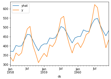
It is easy to see that although the overall trend of the sequence has good fitting results, there is still a large gap in the specific value.

2. Machine learning model. RandomForest model, which is often used as various baseline s, is selected here. When using machine learning to realize time series prediction, it is usually necessary to extract features and labels by sliding windows, and then in fact, it is also necessary to slide the intercepted test set features to realize one-step prediction. Referring to the practice in the paper Machine Learning Strategies for Time Series Forecasting, this problem can be roughly described as follows:

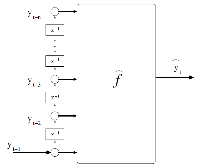
Accordingly, set the length of the feature extraction window to 12, and build the training set and test set as follows:

data = df.copy()
n = 12
for i in range(1, n+1):
    data['ypre_'+str(i)] = data['y'].shift(i)
data = data[['ds']+['ypre_'+str(i) for i in range(n, 0, -1)]+['y']]

# Extract training set and test set
X_train = data[data['ds']<"19580101"].dropna()[['ypre_'+str(i) for i in range(n, 0, -1)]]
y_train = data[data['ds']<"19580101"].dropna()[['y']]
X_test = data[data['ds']>="19580101"].dropna()[['ypre_'+str(i) for i in range(n, 0, -1)]]
y_test = data[data['ds']>="19580101"].dropna()[['y']]

# Model training and prediction
rf = RandomForestRegressor(n_estimators=10, max_depth=5)
rf.fit(X_train, y_train)
y_pred = rf.predict(X_test)

# Result comparison drawing
y_test.assign(yhat=y_pred).plot()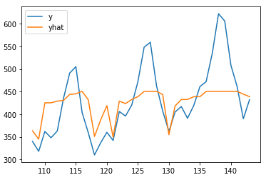

It can be seen that the prediction effect is also relatively general, especially for the prediction results in the last two years, there is a large gap with the real value. It is easy to explain this phenomenon with the thinking of machine learning model: the random forest model is actually learning the law between curves according to the training data set. Because the time series shows an overall growth trend with time, the highest point in the historical data is not enough to cover the larger value in the future, Therefore, all labels that exceed the historical data in the test set are actually unable to fit.

3. For the cyclic neural network in deep learning, in fact, deep learning generally requires a large data set to give full play to its advantages, and the data set here is obviously very small, so only one simplest model is designed: 1-layer LSTM+1-layer Linear. The model is built as follows:

class Model(nn.Module):
    def __init__(self):
        super().__init__()
        self.rnn = nn.LSTM(input_size=1, hidden_size=10, batch_first=True)
        self.linear = nn.Linear(10, 1)
        
    def forward(self, x):
        x, _ = self.rnn(x)
        x = x[:, -1, :]
        x = self.linear(x)
        return x

The construction idea of the data set is the same as the machine learning part mentioned above. Then, the alchemy is trained according to the model. Some results are as follows:

# Convert dataset to 3D
X_train_3d = torch.Tensor(X_train.values).reshape(*X_train.shape, 1)
y_train_2d = torch.Tensor(y_train.values).reshape(*y_train.shape, 1)
X_test_3d = torch.Tensor(X_test.values).reshape(*X_test.shape, 1)
y_test_2d = torch.Tensor(y_test.values).reshape(*y_test.shape, 1)

# Model, optimizer, evaluation criteria
model = Model()
creterion = nn.MSELoss()
optimizer = optim.Adam(model.parameters())

# Training process
for i in range(1000):
    out = model(X_train_3d)
    loss = creterion(out, y_train_2d)
    optimizer.zero_grad()
    loss.backward()
    optimizer.step()
    
    if (i+1)%100 == 0:
        y_pred = model(X_test_3d)
        loss_test = creterion(y_pred, y_test_2d)
        print(i, loss.item(), loss_test.item())

# Training results
99 65492.08984375 188633.796875
199 64814.4375 187436.4375
299 64462.09765625 186815.5
399 64142.70703125 186251.125
499 63835.5 185707.46875
599 63535.15234375 185175.1875
699 63239.39453125 184650.46875
799 62947.08203125 184131.21875
899 62657.484375 183616.203125
999 62370.171875 183104.671875

Through the above 1000 epoch s, it can be inferred that the model will not fit well, so give up decisively!

Of course, it must be pointed out that the above test results can only explain the performance of the three schemes on the data set, but can not represent the performance of this kind of model in time series prediction. In fact, the time series prediction problem itself is a scene requiring specific analysis of specific problems. There is no universal good model, just like "No Free Lunch"!

This article is just a small test of a series of tweets on time series prediction. Other relevant experiences and summaries will be updated from time to time.