Random forest algorithm and ensemble learning - panden's Machine Learning notes

The book continues, Classic decision trees CART, ID3 and C4.5 , we build a tree to solve the problems of classification and fitting, but the disadvantage of a tree is also obvious, that is, it is easy to over fit; Besides, even if a tree is strong, it can't be stronger than several. It's the so-called three Zhuge Liang top a smelly cobbler... And the random forest is such a forest composed of many small trees. The core idea is to let each small tree vote;

Aggregation model

Same weight

G ( X ) = s i g n ( ∑ t = 1 T 1 ∗ g t ( x ) ) G(X) = sign(\sum_{t=1}^T 1*g_t(x)) G(X)=sign(t=1∑T​1∗gt​(x))

Variable interpretation:

• G ( X ) G(X) G(X) represents the final result, s i g n sign sign is a judgment symbol function, and the final judgment is 0 or 1
• g t ( x ) g_t(x) gt (x) represents the prediction result given by each small tree
• ∑ \sum Σ followed by 1 represents the weight of each small tree

Different weights

G ( X ) = s i g n ( ∑ t = 1 T α t ∗ g t ( x ) ) G(X) = sign(\sum_{t=1}^T \alpha_t*g_t(x)) G(X)=sign(t=1∑T​αt​∗gt​(x))

Among them, α t \alpha_t α T ， indicates the weight of the t-th small tree. The reason for this setting is to believe that some trees may have unexpected results, because sometimes when voting in the village, the respected village head may be able to vote twice;

How to generate g ( x ) g(x) g(x)

Because the aggregation model needs many different small trees, the problem we need to solve now is how to generate different small trees under the same set of data?

• Use the same data, but with different hyperparameters
• The same super parameter, different samples (the same data, but not all samples, part)
• The same super parameter and different attributes (the same data, but some small trees only give some attributes)
• The same hyperparameters, the same samples and attributes, but the data weights are different

For the decision tree algorithm, g ( t ) g(t) There are also two ideas for the composition of g(t):

Bagging (one bag model)

The training set is sampled, and the sampling results are used for the training set g ( x ) g(x) g(x), parallel and independent training; Such as random forest.

Boosting (lifting model)

Using the model trained by the training set, adjust the training set according to the prediction results of this training, and then use the adjusted training set to train the next model, serial; Such as adaboost, GBDT, xgbost.

Note: Bagging and Boosting are integrated learning ideas that can be used in any algorithm of machine learning, such as:

Random forest

The random forest is the class of Uniform Blending Voting for Classification in the aggregation model

Idea: Bagging idea + decision tree as base model (each small tree is fully gorwn CART) + Uniform Blending Voting

• Remember the sign in front?

In the random forest, sign is understood as the minority obeys the majority. If there are 100 small trees, the final result of small trees voting is positive example: negative example = 60:40, then the final result after sign is 1;

• characteristic:
  • Efficient parallel
  • Inherit the advantages of decision tree
  • Reduce the over fitting problem of decision tree

Out of bag data

Because the small tree is sampled randomly, there will be no extracted data

The number of data samples is m, and the probability that a data m round is not drawn is
( 1 − 1 m ) m (1-\frac{1}{m})^m (1−m1​)m

When m approaches infinity
lim ⁡ m → ∞ ( 1 − 1 m ) m = 1 e \lim_{m\to\infty}(1-\frac{1}{m})^m = \frac{1}{e} m→∞lim​(1−m1​)m=e1​

So in a random forest with a large sample and many small trees, there will always be 1 e \frac{1}{e} The samples of e1 ＾ will not be included in the training set, and these data can be used as the test set;

Therefore, when using random forest, there is no need to divide the data set, and the OOB of random forest can be self verified;

Actual iris data set

Multiple models + bagging

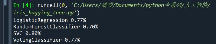
Compare logistic regression, random forest, SVM and bagging the previous three models

from sklearn.ensemble import RandomForestClassifier
from sklearn.ensemble import VotingClassifier
from sklearn.linear_model import LogisticRegression
from sklearn.svm import SVC
from sklearn.datasets import load_iris
from sklearn.model_selection import train_test_split
from sklearn.ensemble import BaggingClassifier
from sklearn.tree import DecisionTreeClassifier
from sklearn.metrics import accuracy_score

#VotingClassifier
log_clf = LogisticRegression()
rnd_clf = RandomForestClassifier()
svm_clf = SVC()

voting_clf = VotingClassifier(
    estimators=[('lr', log_clf), ('rf', rnd_clf), ('svc', svm_clf)],
    voting='hard'  #hard said that in addition to voting, soft takes the result of the classifier with the most certain classification (the highest probability) as the final result
)

iris = load_iris()
X = iris.data[:, :2]  # Calyx length and width
y = iris.target
X_train, X_test, y_train, y_test = train_test_split(X, y, test_size=0.2, random_state=2)

# voting_clf.fit(X, y)


for clf in (log_clf, rnd_clf, svm_clf, voting_clf):
    clf.fit(X_train, y_train)
    y_pred = clf.predict(X_test)
    print(clf.__class__.__name__,'%.2f%%' %accuracy_score(y_test, y_pred))

• The results are as follows:

Shows the error rate

Random forest OOB

The above method is to divide the test set and training set, while the random forest does not need to be divided, so you can verify it yourself

#%%BaggingClassifier
iris = load_iris()
X = iris.data[:, :2]  # Calyx length and width
y = iris.target


bag_clf = BaggingClassifier(
    DecisionTreeClassifier(), n_estimators=10,
    max_samples=1.0, bootstrap=True, n_jobs=1
)
#Accuracy of dividing training set and test set
bag_clf.fit(X_train, y_train)
y_pred = bag_clf.predict(X_test)
print(y_pred)
y_pred_proba = bag_clf.predict_proba(X_test)
print(y_pred_proba)
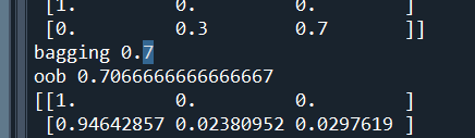
print("bagging", accuracy_score(y_test, y_pred)) #View accuracy


# oob (use the characteristics of random forest to check the accuracy)
bag_clf = BaggingClassifier(
    DecisionTreeClassifier(), n_estimators=500,   #n_estimators represent 500 families of small trees
    bootstrap=True, n_jobs=1, oob_score=True      #bootstrap has been put back for sampling
)
bag_clf.fit(X, y)
print('oob',bag_clf.oob_score_)
# y_pred = bag_clf.predict(X_test)
# print(accuracy_score(y_test, y_pred))

print(bag_clf.oob_decision_function_)  #With y above_ pred_ Proba works similarly, except that there is no need for a test set

• The verification results of test set and OOB are used respectively

The former is the result of the division of test set and training set, and the latter is the way of OOB. There is little difference between the two

Random forest algorithm and ensemble learning, continue to the next chapter! pd's Machine Learning