Support vector machine
Support vector machine (SVM) is a very powerful and flexible supervised learning algorithm, which can be used for both classification and regression. In this section, we will introduce the principle of support vector machine and use it to solve the classification problem. First, import the required Library:
%matplotlib inline
import numpy as np
import matplotlib.pyplot as plt
from scipy import stats
#Drawing with Seaborn
import seaborn as sns; sns.set()
Discriminant classification will be introduced here
Methods: instead of modeling each type of data, a split line (line or curve in two-dimensional space) or flow shape is used
(generalization of the concepts of curves and surfaces in multidimensional space) separate various types.
The following is a simple classification example, in which two types of data can be clearly separated
%matplotlib inline
import numpy as np
import matplotlib.pyplot as plt
from scipy import stats
# Drawing with Seaborn
import seaborn as sns; sns.set()
from sklearn.datasets.samples_generator import make_blobs
X, y = make_blobs(n_samples=50, centers=2,
random_state=0, cluster_std=0.60)
plt.scatter(X[:, 0], X[:, 1], c=y, s=50, cmap='autumn');
E:\anaconda3\lib\site-packages\sklearn\utils\deprecation.py:143: FutureWarning: The sklearn.datasets.samples_generator module is  deprecated in version 0.22 and will be removed in version 0.24. The corresponding classes / functions should instead be imported from sklearn.datasets. Anything that cannot be imported from sklearn.datasets is now part of the private API.
  warnings.warn(message, FutureWarning)

This linear discriminant classifier attempts to draw a straight line that divides the data into two parts, which constitutes a classification model.
For the two-dimensional data in the figure above, this task can be completed manually. But we immediately found a problem: in
Between these two types, there is more than one straight line that can perfectly divide them.
xfit = np.linspace(-1, 3.5)
plt.scatter(X[:, 0], X[:, 1], c=y, s=50, cmap='autumn')
plt.plot([0.6], [2.1], 'x', color='red', markeredgewidth=2, markersize=10)
for m, b in [(1, 0.65), (0.5, 1.6), (-0.2, 2.9)]:
    plt.plot(xfit, m * xfit + b, '-k')
plt.xlim(-1, 3.5);
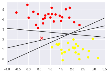
Although these three different dividers can distinguish these samples perfectly, choosing different segmentation lines may make the new
Data points are assigned to different labels. Obviously, "draw a line to separate different types
"Straight line" is not enough, we need to think further.
Support vector machines: boundary maximization
Support vector machine provides a way to improve this problem. Its intuitive explanation is that it no longer draws a thin line to distinguish classification
Type, but draw a line with width to the nearest point boundary.
xfit = np.linspace(-1, 3.5)
plt.scatter(X[:, 0], X[:, 1], c=y, s=50, cmap='autumn')
for m, b, d in [(1, 0.65, 0.33), (0.5, 1.6, 0.55), (-0.2, 2.9, 0.2)]:
    yfit = m * xfit + b
    plt.plot(xfit, yfit, '-k')
    plt.fill_between(xfit, yfit - d, yfit + d, edgecolor='none', color='#AAAAAA',
    alpha=0.4)
plt.xlim(-1, 3.5);
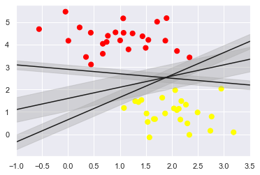
In support vector machine, the line with the largest boundary is the optimal solution of the model. Support vector machine is actually a boundary maximization evaluator.
1. Fitting support vector machine
Let's take a look at the real fitting result of this data: use scikit learn's support vector machine classifier to train one on the data
SVM model. Here we use a linear kernel function and set the parameter C to a large number (these settings will be described later)
Meaning of setting:
from sklearn.svm import SVC # "Support vector classifier"
model = SVC(kernel='linear', C=1E10)
model.fit(X, y)
SVC(C=10000000000.0, kernel='linear')
In order to achieve better visual classification effect, an auxiliary function is created to draw the decision boundary of SVM
def plot_svc_decision_function(model, ax=None, plot_support=True):
#"" "draw decision function for 2D SVC" ""
    if ax is None:
        ax = plt.gca()
    xlim = ax.get_xlim()
    ylim = ax.get_ylim()
    # Create a grid for the evaluation model
    x = np.linspace(xlim[0], xlim[1], 30)
    y = np.linspace(ylim[0], ylim[1], 30)
    Y, X = np.meshgrid(y, x)
    xy = np.vstack([X.ravel(), Y.ravel()]).T
    P = model.decision_function(xy).reshape(X.shape)
    # Draw decision boundaries and boundaries
    ax.contour(X, Y, P, colors='k',levels=[-1, 0, 1], alpha=0.5,linestyles=['--', '-', '--'])
    # Draw support vector
    if plot_support:
        ax.scatter(model.support_vectors_[:, 0],
            model.support_vectors_[:, 1],
            s=300, linewidth=1, facecolors='none');
    ax.set_xlim(xlim)
    ax.set_ylim(ylim)
plt.scatter(X[:, 0], X[:, 1], c=y, s=50, cmap='autumn')
plot_svc_decision_function(model);

This is the dividing line with the largest interval between the two types of data. You will find some points right on the boundary line, in the figure below
Represented by a black circle. These points are the key support points of fitting, which are called support vector, and the support vector machine algorithm is also obtained
Name. In scikit learn, the coordinates of the support vector are stored in the support of the classifier_ vectors_ Properties:
model.support_vectors_
array([[0.44359863, 3.11530945],
       [2.33812285, 3.43116792],
       [2.06156753, 1.96918596]])
The key factor for the classifier to fit successfully is the position of these support vectors - any far away from the correct classification side
Points away from the boundary line will not affect the fitting result! From a technical point of view, it is because these points will not affect the fitting modulus
The type loss functions have no effect, so as long as they do not cross the boundary line, their location and quantity are irrelevant
Close it tightly.
For example, the fitting results of the first 60 points and the first 120 points of the data set can be drawn and compared
def plot_svm(N=10, ax=None):
    X, y = make_blobs(n_samples=N, centers=2,random_state=0, cluster_std=0.60)
    X = X[:N]
    y = y[:N]
    model = SVC(kernel='linear', C=1E10)
    model.fit(X, y)
    ax = ax or plt.gca()
    ax.scatter(X[:, 0], X[:, 1], c=y, s=50, cmap='autumn')
    ax.set_xlim(-1, 4)
    ax.set_ylim(-1, 6)
    plot_svc_decision_function(model, ax)

fig, ax = plt.subplots(1, 2, figsize=(16, 6))
fig.subplots_adjust(left=0.0625, right=0.95, wspace=0.1)
for axi, N in zip(ax, [60, 120]):
    plot_svm(N, axi)
    axi.set_title('N = {0}'.format(N))
[the external chain picture transfer fails. The source station may have an anti-theft chain mechanism. It is recommended to save the picture and upload it directly (img-RowYYAzU-1638086107264)(output_13_0.png)]
What we see in the left figure is the model and support vector of the first 60 training samples. In the right picture, although we draw the front
The support vectors of 120 training samples, but the model has not changed: the three support vectors in the left figure are still applicable to the right
Figure. This feature of being insensitive to data points far from the boundary is one of the advantages of SVM model.
If you are running Notebook, you can use the interactive component of IPython to dynamically observe this feature of SVM model:
from ipywidgets import interact, fixed

interact(plot_svm, N=[10,50,100,200,400,1000], ax=fixed(None));
interactive(children=(Dropdown(description='N', options=(10, 50, 100, 200, 400, 1000), value=10), Output()), _...
2. Beyond the linear boundary: kernel function SVM model
The combination of SVM model and kernel function will be very powerful. We introduced some kernel functions when we introduced basis function regression in section 5.6. At that time, we project the data into the high-dimensional space defined by polynomial and Gaussian basis function, so as to fit the nonlinear relationship with linear classifier.
In the SVM model, we can follow the same idea. In order to apply the kernel function, some nonlinear separable data are introduced:
from sklearn.datasets.samples_generator import make_circles
X, y = make_circles(100, factor=.1, noise=.1)
clf = SVC(kernel='linear').fit(X, y)
plt.scatter(X[:, 0], X[:, 1], c=y, s=50, cmap='autumn')
plot_svc_decision_function(clf, plot_support=False);
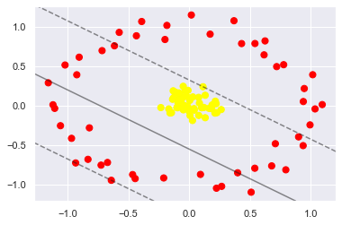
Obviously, nonlinear discriminant method is needed to segment data. For example, a simple cast
The shadow method is to calculate a radial basis function centered on the middle cluster:
r = np.exp(-(X ** 2).sum(1))
You can visualize the new dimensions through three-dimensional graphics - if you are running Notebook, you can use the slider to transform the view
Viewing angle:
from mpl_toolkits import mplot3d
from ipywidgets import interact, fixed

def plot_3D(elev=30, azim=30, X=X, y=y):
    ax = plt.subplot(projection='3d')
    ax.scatter3D(X[:,0], X[:,1], r, c=y, s=50, cmap='autumn')
    ax.view_init(elev=elev, azim=azim)
    ax.set_xlabel('x1')
    ax.set_ylabel('x2')
    ax.set_zlabel('r')

interact(plot_3D, elev=(-90,90), azip=(-180,180), X=fixed(X), y=fixed(y))
interactive(children=(IntSlider(value=30, description='elev', max=90, min=-90), IntSlider(value=30, descriptio...


<function __main__.plot_3D(elev=30, azim=30, X=array([[-5.61706135e-02, -1.91757887e-02],
       [-3.24732855e-02,  1.85784593e-01],
       [-8.34778451e-02,  1.63126655e-01],
       [ 4.88316811e-03,  6.81508121e-02],
       [ 1.88120125e-01,  1.01202439e-02],
       [-9.24798126e-01,  3.93319002e-01],
       [ 2.98673214e-02,  1.12220257e-01],
       [-9.33903161e-01, -7.25906019e-01],
       [ 1.13785077e-01,  2.41229726e-01],
       [ 6.78684592e-01, -7.63475049e-01],
       [ 7.77233896e-02,  1.06533516e-01],
       [ 5.39739473e-01, -7.93135623e-01],
       [-9.54433932e-02, -2.52511525e-02],
       [-9.67876854e-01, -4.13583329e-01],
       [ 9.94196096e-01, -2.42882635e-01],
       [-1.27347610e-01,  1.04114172e-01],
       [-1.36814783e-01,  8.20177861e-02],
       [-2.09592206e-01, -9.16765257e-01],
       [-1.14597190e-02, -1.17949877e-02],
       [ 7.95014208e-01, -8.13113364e-01],
       [-4.91262045e-02, -4.33910038e-02],
       [-9.22485045e-02,  3.55221030e-02],
       [ 7.84815145e-02, -1.22921933e-01],
       [ 1.76821029e-02,  1.15214114e+00],
       [-1.05900323e+00, -2.53303895e-01],
       [ 2.15163839e-01,  5.80610131e-02],
       [-6.76190117e-02,  4.26077146e-02],
       [-1.67978685e-01, -4.02186472e-02],
       [ 4.28001663e-05, -6.98594415e-02],
       [ 7.77284598e-01,  5.21271083e-01],
       [-9.64379469e-03,  1.95547099e-01],
       [ 2.24306831e-01, -1.04671812e+00],
       [-3.12124595e-02, -1.67838209e-02],
       [ 3.68501771e-01,  1.07950178e+00],
       [-1.57760811e-01, -9.18202668e-02],
       [-3.90698563e-01,  1.06957888e+00],
       [-4.72686618e-02, -5.18980575e-02],
       [-8.26677199e-02,  8.43784712e-02],
       [ 2.63302819e-01, -4.83233738e-02],
       [ 2.12089190e-01, -9.32226929e-02],
       [ 6.24169305e-01,  8.23429663e-01],
       [ 1.63485539e-01, -3.28810918e-02],
       [ 5.41091106e-01,  7.90204843e-01],
       [ 9.28014579e-02, -8.71505013e-01],
       [ 2.67106302e-01, -1.02325022e+00],
       [ 4.16526261e-02, -5.59186555e-02],
       [ 1.09454320e+00,  1.49198601e-02],
       [ 9.00094689e-01, -3.95140378e-01],
       [ 2.72264784e-02, -1.86920081e-01],
       [ 2.21751048e-01,  2.63053069e-02],
       [ 2.27910639e-01, -8.75968297e-02],
       [-8.25540328e-02,  1.57331194e-01],
       [ 5.09785794e-01, -1.09760031e+00],
       [ 9.39007013e-01,  5.36068409e-02],
       [-4.65392116e-01, -8.73931995e-01],
       [-7.24910365e-01, -7.53796011e-01],
       [-1.83318038e-01,  1.02028558e+00],
       [ 1.02214812e-01, -2.58856384e-02],
       [ 6.95003485e-03, -1.24334603e-01],
       [ 1.03549068e+00, -4.02378008e-02],
       [-1.15915425e+00,  2.91307649e-01],
       [-4.34428138e-01,  8.88369780e-01],
       [ 8.41760873e-02,  3.38849398e-02],
       [-1.99128729e-01,  8.41339639e-01],
       [-6.14729381e-01,  7.61142681e-01],
       [-1.12062508e+00,  1.25801406e-02],
       [ 3.98666815e-01, -8.50842819e-01],
       [-8.21165857e-01, -2.80405574e-01],
       [-5.75718279e-01,  9.31872289e-01],
       [-1.02142079e+00,  5.17278493e-01],
       [-4.44518201e-01, -9.24758922e-01],
       [-5.19374699e-02,  1.02721828e-01],
       [ 7.08872958e-01, -4.81867406e-01],
       [-2.33096995e-01, -2.32733908e-02],
       [ 1.31870856e-01, -1.51813572e-01],
       [-1.10660504e+00, -3.31377944e-02],
       [ 1.20969414e-01, -2.15979300e-02],
       [ 4.03106177e-02, -3.63263801e-02],
       [-6.45741599e-03, -3.74165685e-02],
       [ 1.85344268e-01, -3.71446375e-02],
       [-1.01641536e-01, -2.32750499e-02],
       [-9.05201532e-01,  6.16640720e-01],
       [-4.91533549e-02,  2.47194062e-01],
       [ 9.46702602e-01,  2.18737482e-01],
       [ 9.37495115e-01, -5.06247325e-01],
       [-3.81712748e-02,  4.11198862e-03],
       [ 1.01615435e+00,  3.94018604e-01],
       [ 7.19813746e-01,  4.97003099e-01],
       [ 1.72205681e-01,  9.09045304e-01],
       [-6.40769531e-01, -9.46126502e-01],
       [ 4.31144691e-01,  7.89412882e-01],
       [-1.11985695e-01,  1.71534587e-01],
       [-2.12194657e-02,  1.22242578e-01],
       [-7.16770280e-01,  6.99875703e-01],
       [ 6.16124161e-01,  6.46132966e-01],
       [-8.32708000e-01, -6.80375210e-01],
       [-1.31598272e-01,  1.89920315e-01],
       [-6.72098659e-01, -7.19958362e-01],
       [ 1.31784847e-01,  1.33165268e-01],
       [-1.45684274e-01, -8.82333984e-02]]), y=array([1, 1, 1, 1, 1, 0, 1, 0, 1, 0, 1, 0, 1, 0, 0, 1, 1, 0, 1, 0, 1, 1,
       1, 0, 0, 1, 1, 1, 1, 0, 1, 0, 1, 0, 1, 0, 1, 1, 1, 1, 0, 1, 0, 0,
       0, 1, 0, 0, 1, 1, 1, 1, 0, 0, 0, 0, 0, 1, 1, 0, 0, 0, 1, 0, 0, 0,
       0, 0, 0, 0, 0, 1, 0, 1, 1, 0, 1, 1, 1, 1, 1, 0, 1, 0, 0, 1, 0, 0,
       0, 0, 0, 1, 1, 0, 0, 0, 1, 0, 1, 1], dtype=int64))>
After adding a new dimension, the data becomes linearly separable. If you now draw a split plane, for example, r = 0.7, that is
Data can be split.
We also need to carefully select and optimize the projection mode; If the radial basis function cannot be concentrated in the correct position, then
Can't get such a clean and divisible result. Usually, it is difficult to select the basis function. We need to let the model point out automatically
The most appropriate basis function.
One strategy is to calculate the transformation results of each point of the basis function on the data set, and let the SVM algorithm filter out all the results
Optimal solution. This basis function transformation is called kernel transformation, which is based on the similarity (or kernel function) between each pair of data points
Number) calculated.
The problem with this strategy is that if N data points are projected into N-dimensional space, it will appear when N is increasing
Dimension disaster, huge amount of calculation. But due to kernel technique http://bit.ly/2fStZeA
The applet provided can be implicit
Calculate the fitting of kernel transformation data, that is, there is no need to establish a complete N-dimensional kernel function projection space! This kernel function
The technique built into the SVM model is a sufficient condition for making the SVM method so powerful.
In scikit learn, we can use the kernel function SVM model to transform the linear kernel into RBF (radial basis function)
Number of cores, and set the kernel model super parameters:
clf = SVC(kernel='rbf', C=1E6)
clf.fit(X, y)
SVC(C=1000000.0)
plt.scatter(X[:, 0], X[:, 1], c=y, s=50, cmap='autumn')
plot_svc_decision_function(clf)
plt.scatter(clf.support_vectors_[:, 0], clf.support_vectors_[:, 1],
s=300, lw=1, facecolors='none');
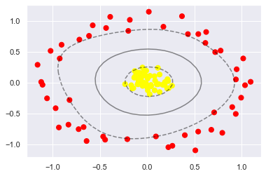
By using this kernel based support vector machine, we find a suitable nonlinear decision boundary. In Machine Science
In practice, kernel transformation strategy is often used to transform fast linear methods into fast nonlinear methods, especially for those who can
Model using kernel function technique.
3.SVM Optimization: softening boundary
So far, the models we have introduced are all dealing with very clean data sets, in which there are very perfect decisions
Boundary. But what if your data has some overlap? For example, there are some data as follows:
X, y = make_blobs(n_samples=100, centers=2,
random_state=0, cluster_std=1.2)
plt.scatter(X[:, 0], X[:, 1], c=y, s=50, cmap='autumn');

In order to solve this problem, SVM implements some correction factors to "soften" the boundary. In order to obtain better fitting effect
As a result, it allows some points to be located within the boundary line. The hardness of the boundary line can be controlled by super parameters, usually C.
If C is large, the boundary will be hard, and data points cannot "survive" within the boundary; If C is small, the boundary line ratio
Soft, some data points can cross the boundary line.
X, y = make_blobs(n_samples=100, centers=2,
                    random_state=0, cluster_std=0.8)
fig, ax = plt.subplots(1, 2, figsize=(16, 6))
fig.subplots_adjust(left=0.0625, right=0.95, wspace=0.1)
for axi, C in zip(ax, [10.0, 0.1]):
    model = SVC(kernel='linear', C=C).fit(X, y)
    axi.scatter(X[:, 0], X[:, 1], c=y, s=50, cmap='autumn')
    plot_svc_decision_function(model, axi)
    axi.scatter(model.support_vectors_[:, 0],
        model.support_vectors_[:, 1],
        s=300, lw=1, facecolors='none');
axi.set_title('C = {0:.1f}'.format(C), size=14)
Text(0.5, 1.0, 'C = 0.1')

Case: face recognition
We use face recognition cases to demonstrate the practical process of support vector machine. Here we use the labeled face in the Wild dataset
Image, which contains thousands of public face photos. Scikit learn has built-in function to obtain photo data sets:
from sklearn.datasets import fetch_lfw_people
faces = fetch_lfw_people(min_faces_per_person=60)
print(faces.target_names)
print(faces.images.shape)
['Ariel Sharon' 'Colin Powell' 'Donald Rumsfeld' 'George W Bush'
 'Gerhard Schroeder' 'Hugo Chavez' 'Junichiro Koizumi' 'Tony Blair']
(1348, 62, 47)
fig, ax = plt.subplots(3, 5)
for i, axi in enumerate(ax.flat):
    axi.imshow(faces.images[i], cmap='bone')
    axi.set(xticks=[], yticks=[],
            xlabel=faces.target_names[faces.target[i]])

Each image contains [62] × 47], close to 3000 pixels. Although each pixel can be simply regarded as a feature, but
Is a more efficient method, usually using a preprocessor to extract more meaningful features. Principal component analysis (PCA) is used here
See section 5.9) to extract 150 basic elements and provide them to the support vector machine classifier. You can put this
The preprocessor and classifier are packaged into a pipeline:
from sklearn.svm import SVC
# from sklearn.decomposition import RandomizedPCA
from sklearn.decomposition import PCA as RandomizedPCA
from sklearn.pipeline import make_pipeline

pca = RandomizedPCA(n_components=150, whiten=True, random_state=42)
svc = SVC(kernel='rbf', class_weight='balanced')
model = make_pipeline(pca, svc)
In order to test the training effect of the classifier, the data set is decomposed into training set and test set for cross inspection:
from sklearn.model_selection import train_test_split
Xtrain, Xtest, ytrain, ytest = train_test_split(faces.data, faces.target,
    random_state=42)
Xtrain
array([[107.333336, 107.333336, 108.666664, ..., 109.      ,  96.333336,
         99.      ],
       [ 90.666664,  63.      ,  57.666668, ..., 216.33333 , 218.      ,
        218.      ],
       [134.66667 , 124.333336, 129.      , ..., 158.      , 165.      ,
        171.66667 ],
       ...,
       [ 73.333336,  53.333332,  48.666668, ...,  40.666668,  71.333336,
         80.666664],
       [ 52.      ,  94.333336, 121.333336, ..., 252.      , 251.66667 ,
        250.33333 ],
       [157.66667 , 141.66667 , 133.      , ...,  12.      ,  11.      ,
          8.333333]], dtype=float32)
By continuously adjusting parameter C (control the hardness of the boundary line)
Degree) and parameter gamma (controlling the size of radial basis function kernel) to determine the optimal model:
from sklearn.model_selection import GridSearchCV
param_grid = {'svc__C': [1, 5, 10, 50],
            'svc__gamma': [0.0001, 0.0005, 0.001, 0.005]}
grid = GridSearchCV(model, param_grid)
%time grid.fit(Xtrain, ytrain)
print(grid.best_params_)
Wall time: 31.7 s
{'svc__C': 10, 'svc__gamma': 0.001}
The optimal parameters finally fall in the middle of the grid. If they fall on the edge, we may need to expand the network
Lattice search range to ensure that the optimal parameters can be searched.
With the cross check model, you can now predict the data of the test set:
model = grid.best_estimator_
yfit = model.predict(Xtest)
Compare some test pictures with prediction pictures
fig, ax = plt.subplots(4, 6)
for i, axi in enumerate(ax.flat):
    axi.imshow(Xtest[i].reshape(62, 47), cmap='bone')
    axi.set(xticks=[], yticks=[])
    axi.set_ylabel(faces.target_names[yfit[i]].split()[-1],
                        color='black' if yfit[i] == ytest[i] else 'red')
fig.suptitle('Predicted Names; Incorrect Labels in Red', size=14);
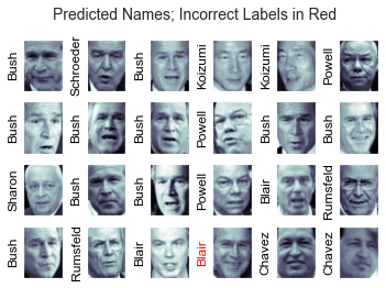
In this small sample, our optimal evaluator only misjudged one picture (Bush's picture in the last line was misjudged)
For Blair). We can print the classification effect report, which lists the statistical results of each label, so as to evaluate the evaluator
Have a more comprehensive understanding of the performance of:
from sklearn.metrics import classification_report
print(classification_report(ytest, yfit,target_names=faces.target_names))
                   precision    recall  f1-score   support

     Ariel Sharon       0.65      0.73      0.69        15
     Colin Powell       0.80      0.87      0.83        68
  Donald Rumsfeld       0.74      0.84      0.79        31
    George W Bush       0.92      0.83      0.88       126
Gerhard Schroeder       0.86      0.83      0.84        23
      Hugo Chavez       0.93      0.70      0.80        20
Junichiro Koizumi       0.92      1.00      0.96        12
       Tony Blair       0.85      0.95      0.90        42

         accuracy                           0.85       337
        macro avg       0.83      0.84      0.84       337
     weighted avg       0.86      0.85      0.85       337
from sklearn.metrics import confusion_matrix
mat = confusion_matrix(ytest, yfit)
sns.heatmap(mat.T, square=True, annot=True, fmt='d', cbar=False,
            xticklabels=faces.target_names,
            yticklabels=faces.target_names)
plt.xlabel('true label')
plt.ylabel('predicted label');

This picture can help us clearly judge which tags are easy to be misjudged by the classifier.
Photos of face recognition problems in real environment are usually not cut so neatly (even if the pixels are the same), two kinds of people
The only difference between face classification mechanisms is actually feature selection: you need to use more complex algorithms to find faces and then extract images
Face features independent of pixelation in. A good solution to such problems is to use OpenCV (http://
opencv.org) in conjunction with other means, including the most advanced feature extraction tools for general images and face images
Face feature data.
Support vector machine summary
The basic principles of support vector machine have been briefly introduced. Support vector machine is a powerful classification method for four main reasons.
- The model relies on relatively few support vectors, indicating that they are very exquisite models and consume less memory.
- Once the model training is completed, the prediction phase is very fast.
- Because the models are only affected by the points near the boundary line, they have a very good learning effect for high-dimensional data - even training data higher than the sample dimension is no problem, which is difficult for other algorithms.
- The cooperation with kernel function method is very universal and can be applied to different types of data. However, SVM model also has some disadvantages.
- With the increasing sample size N, the worst training time complexity will reach O [ N 3 ] {O[N^3]} O[N3]; After efficient treatment, it can only reach O [ N 2 ] {O[N^2]} O[N2]. Therefore, the computational cost of large sample learning will be very high.
- The training effect depends on whether the boundary softening parameter C is reasonable or not. This requires self searching through cross checking; When the data set is large, the amount of calculation is also very large.
- The prediction results cannot be explained by probability directly. This can be evaluated by internal cross test (see the definition of SVC's probability parameter for details), but the evaluation process also requires a lot of calculation.
Due to these limitations, I usually choose support vector machine only when other simple, fast and less difficult methods can not meet the requirements. However, if your computing resources are enough to support SVM training and cross checking of data sets, you can get excellent results with it.
The performance of SVM in weak learners has always been very superior, but in this era, it is recommended to use better algorithms. Mainly integrated algorithms, such as random forest and XGBoost. stay kaggle There are basically integration algorithms, ha ha.