abstract
Passenger flow forecast of urban rail transit is the main basis for decision-making of rail transit construction scale, and plays an important role in project design.
With the construction and development of rail transit in China, subway has become an important way of public travel. When important events such as holidays, competitions and performances occur, subway passenger flow will face great pressure. From the card swiping data of railway gates in Zhengzhou from August to November of a year, the inbound and outbound status can be extracted according to the transaction type. It is necessary to predict the daily passenger flow of each station within 7 days from December 1 to 7 (the transaction type is the sum of 21 and 22 times), so as to provide early warning support for festival security and flow control.
1. Introduction
Urban rail transit project is a project of a century long plan in the city. Therefore, it is necessary to predict the passenger flow scale of rail transit in the coming years and fully reserve the scale of rail transit project, which can not only be used to alleviate the current traffic pressure. Therefore, passenger flow prediction is particularly important.
There is no doubt that passenger flow forecast is the most important special project in the preliminary research of urban rail transit project. It determines the setting scale, facility form, investment and financing of rail transit. However, unlike other research projects, passenger flow forecasting can analyze right and wrong. It is a prediction of the future city for several years. The complexity and uncertainty of urban development increase the risk of passenger flow forecasting.
At present, some domestic rail transit researchers do not pay attention to passenger flow forecasting (they think it is not highly technical and has great errors), and the design scheme is often determined according to their experience. However, such an important special research lacks our reflection. Why is the passenger flow forecasting inaccurate? Is there a problem with the passenger flow forecasting researchers or the basic data, Or there is something wrong with our research methodology (traffic model).
2. Research history of passenger flow forecast at home and abroad
2.1 research history of passenger flow forecast at home and abroad
Marked by the Chicago Area Transportation Study published in Chicago in 1962, the transportation planning theory and method were born, and the four stage prediction theory was put forward for the first time. The federal highway law formulated by the United States in 1962 stipulates that cities with a population of more than 50000 must formulate metropolitan traffic planning based on urban comprehensive traffic survey before they can receive financial subsidies for highway construction from the federal government.
At present, major developed countries in Europe and the United States attach great importance to the establishment and maintenance of traffic prediction models. Some local governments even stipulate the status and importance of traffic prediction models and the income of traffic modelers in the form of local regulations. Major cities have established a set of mature traffic models suitable for their own regions, which are becoming more and more stable and mature with the development of cities, The prediction accuracy is gradually improved.
2.2 comparative analysis of passenger flow forecast research at home and abroad
From the development process of passenger flow forecasting research at home and abroad, the passenger flow forecasting research at home and abroad has a development trend from simple and large error to a gradually perfect and mature traffic forecasting system.
The initial error of foreign passenger flow forecasting research is still large. Simple analysis can be made by the following factors:
(1) The city is developing rapidly, and there is still uncertainty in basic data, especially urban planning and relevant policies
(2) The traffic prediction theory is not mature and is in the exploratory stage;
(3) Traffic modelers have insufficient understanding of the current situation and future passenger flow development trend of the city, and lack experience in modifying and adjusting traffic model parameters suitable for the city.
With the gradual stability of foreign urban development, urban planning, the maturity of traffic model theory and the experience of traffic modelers, the reliability of passenger flow prediction has been brought, and the error of prediction results is becoming smaller and smaller. This has also brought confidence to local authorities, and even issued relevant policies to stipulate that traffic models must be used in the research stage of traffic planning and traffic facilities construction.
3. Complexity analysis of passenger flow forecast
From the development process of passenger flow forecasting at home and abroad, the factors affecting passenger flow forecasting can be divided into three aspects: basic data of passenger flow forecasting, traffic forecasting theory and traffic modeler. The three constitute a complex system of passenger flow forecasting, and each of them is a key factor affecting the accuracy of passenger flow forecasting.
3.1 basic data of passenger flow forecast
The basic data of passenger flow forecast is the input source of the traffic model. Obviously, if the traffic model is regarded as a black box, if the input source itself has errors, the passenger flow forecast results will inevitably produce errors. The collection of basic data of passenger flow forecast is also quite complex, which is mainly divided into four categories:
3.1. 1. Basic information
Basic information mainly includes urban population, employment and socio-economic data. Basic information data is helpful for traffic modelers to study and judge the historical change trend and make reasonable prediction for the next year. It mainly includes the future annual employment rate, time value, etc.
3.1. 2. Traffic investigation
Traffic survey mainly includes resident travel survey, floating population travel survey, urban external access survey, etc. The purpose of traffic survey can not only be used to analyze the passenger flow distribution characteristics of the current city, so as to facilitate the modeler to judge the development characteristics and change trend of urban passenger flow in the future, but also contribute to the calibration of traffic model parameters, In order to establish a traffic model suitable for the city.
3.1. 3 urban planning
Urban planning mainly includes urban master planning, comprehensive traffic planning and special planning. These plans mainly demonstrate and plan the development scale, urban spatial structure, infrastructure distribution and scale of the city in the coming years.
It should be said that the relevant data of urban planning play an important role in the establishment of traffic model in the coming years. The stability, rationality and credibility of its planning are very key, which determines the error of prediction results in the coming years. For a simple example, it is planned that the future population of a new area will be 500000, but the planning year will only accommodate 300000, which will inevitably lead to the error of passenger flow prediction results.
3.2 passenger flow forecasting theory
From the prediction methods adopted at home and abroad, it can be roughly divided into three forms: trend extension method, attraction range method and four-stage method of traffic planning (trend extension method, attraction range method and four-stage method).
The first two methods only consider the changes of passenger flow in the rail line and its attraction range, and do not consider that the completion of the rail transit system as the backbone of the whole urban transportation will lead to the changes of the distribution state of the whole urban passenger flow on the urban road network. It is widely used in the initial stage of passenger flow forecasting research, but it has been rarely used at present.
3.3 traffic Modeler
The traffic modeler cannot be divorced from the passenger flow forecasting system, because he is the traffic data analysis and traffic model builder, which directly determines the accuracy of passenger flow forecasting. In fact, under the premise of the same basic data, different traffic modelers will inevitably have different passenger flow prediction results. Therefore, traffic modelers are also the main reason for the error of passenger flow prediction results.
4. Controllability analysis of passenger flow forecast
Although the passenger flow forecasting system is very complex and involves all aspects, which makes the passenger flow forecasting risky and uncertain, whether the risk is controllable is worth further discussion.
In the passenger flow forecasting system, three factors determine the accuracy of passenger flow forecasting. Among them, the traffic forecasting theory is relatively mature, and the risks and errors in this regard can be measured. At present, there is no better and more advanced forecasting theory.
Therefore, as long as the errors caused by the input end (basic data) and the user end (traffic modeler) are controlled, the risk can be well controlled. In fact, the risk in this aspect is controllable.
Here, the passenger flow forecast of Nanjing Metro Line South extension and line 2 during the opening period is taken as an example to illustrate the controllability of risk.
5. Characteristic analysis of subway passenger flow data
Feature analysis is distinguished from mining features and two dimensions:
Firstly, from the point of view of the station, the daily passenger flow changes are roughly the same as the previous dates of the same type, but what causes the fluctuation. Secondly, from the perspective of users, the behavior trajectory of most users should be repetitive, that is, passenger flow stability. For the two dimensions, in terms of time, distinguish the impact of holidays and peak hours on passenger flow. Spatially, distinguish the impact of passenger flow caused by different geographical locations and functional attributes. Through the above two angles and dimensions, four types of features are summarized, namely, basic features, time features, historical time features and geographic information features.
5.1 overview of function analysis
(1) Basic features: common features are used for passenger flow forecasting under non special circumstances. The construction of conventional features in this paper is to use the common features in passenger flow prediction in the current research, judge passenger flow prediction according to experience, effectively select relevant passenger flow data and quantify relevant qualitative features.
(2) Time characteristics: commute characteristics of normal passenger flow. Include date type and peak time. Data types include working days, weekends and holidays, and peak hours include peacetime, peak hours and special peak hours.
(3) Historical passenger flow characteristics: continuous correlation of passenger flow changes. Passenger flow change is a dynamic and continuous process. The passenger flow at any time is the change of the passenger flow at the previous time.
(4) Geographic information features: mainly describe the geographic information factors that may affect passenger flow.
5.2 basic functions
According to the basic information obtained during data preprocessing, including station ID, day, hour, minute, week, time cutting, number and number. Where, the number in indicates the number of arrivals during this period, and the number out indicates the number of departures during this period.
(1) Basic features: there are many kinds of basic information. Basic stations, weeks, days, hours and minutes are built as basic time information functions.
(2) Time: the period variable t represents the index of the time period obtained by dividing a day by 10 minutes. The objective output of this paper is the prediction of passenger flow within 10 minutes. Since 10 minutes can reflect the change of time and give response time to station operation management, 10 minutes is the fine-grained passenger flow prediction. A day can be divided into 144 parts.
t={0,1,2,......,143}
(3) Week uses W (t) to represent one day of the week.

5.3 time function
For the prediction of urban rail transit passenger flow, the passenger flow will also be affected by common time factors. Therefore, it is necessary to analyze the time influencing factors of traditional passenger flow change, and construct the time characteristics on this basis. The construction basis of time characteristics is as follows.
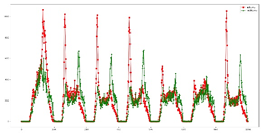
(1) Date type: in terms of time type, it can be divided into three types, especially working days, weekends and holidays (Bai et al., 2017). According to the display in the figure below, we can see that there is a huge difference between weekend passenger flow and ordinary passenger flow. Therefore, weekends and weekdays should be regarded as different functions, which can make the function extraction more in line with the actual functions.
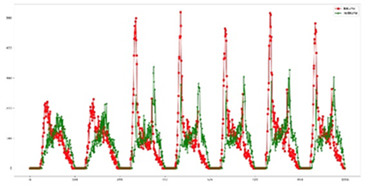
From the following figures, the first day is a holiday. It is easy to see that the passenger flow during the holiday is very different from the usual weekends and ordinary working days.
Therefore, working days, weekends and holidays should be re characterized as date types.
According to the date type, each day is divided into three types: working day, weekend and holiday, which are represented by the characteristic variable F (t).

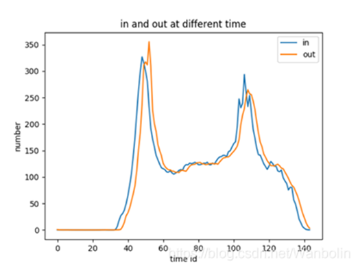
(2) Peak time
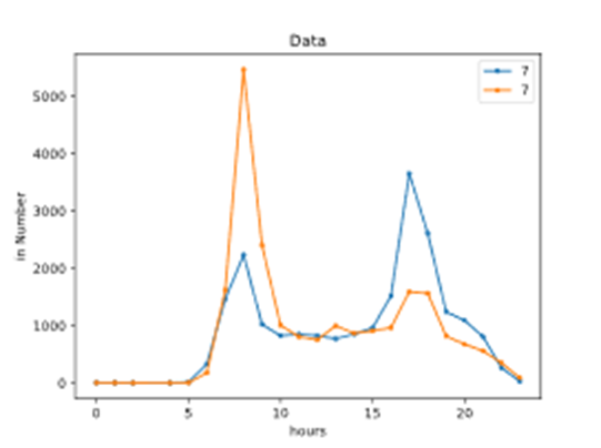
The types of events in a day may have peaks and cycles. As can be seen from the figure below, there are usually two peaks in a day, namely morning peak and evening peak. However, it is worth noting that there are also peaks between the morning and evening peaks. I judge this peak as a special peak.
5.4 historical passenger flow characteristics
Historical passenger flow characteristics, i.e. time window characteristics. The time window function is a more powerful function, because the value of one time is closely related to the value of the previous time. For time series data, short-term weighted values are constructed. By scrolling the time window, the function of short time window with different time will be generated step by step.
(1) Adjacent period
Considering that there is a certain relationship between the traffic information at the current time and the traffic information before and after, the passenger flow is characterized by the traffic information of the first two periods and the last two periods of the current period. In inNums_before1,inNums_before2,inNums_after1,inNums_after2,outNums_before1,outNums_before2,outNums_after1,outNums_ After 2 is the characteristic of passenger flow at the corresponding time.
(2) Adjacent day
The maximum, average and minimum passenger flows reflect the distribution information of the data to a certain extent (Liu et al., 2017), so they are characterized by the maximum, average and minimum inbound and outbound flows in the same week.
(3) The weekly passenger flow is in the previous order
The distribution characteristics can also reflect the outbound passenger flow by using the same station in the same week, the same time period and the same day (Luo, 2017).
5.5 geographic information function
The characteristics of geographic information mainly include station type, station attribute, station equipment, passenger flow stability, etc. Geographic information functions are fully considered when designing all information related to geographic information. Full consideration is given to the geographical location, function, attribute and passenger flow stability.
(1) Station type
Different stations, such as departure station, transfer station and ordinary station. The number of adjacent stations can represent the type of these stations, so the number of adjacent stations is calculated according to the road network diagram to indicate the type of each station. The departure station has only one adjacent station, the ordinary station consists of two adjacent stations, and the transfer station has more than two adjacent stations.
(2) Station properties
Different stations also have different properties. According to different attributes, it can be divided into business attributes, work attributes and residential attributes. According to figure 17, the passenger flow patterns between different stations are quite different. Some stations have more passengers on weekends than on weekdays, so they can be judged as commercial.
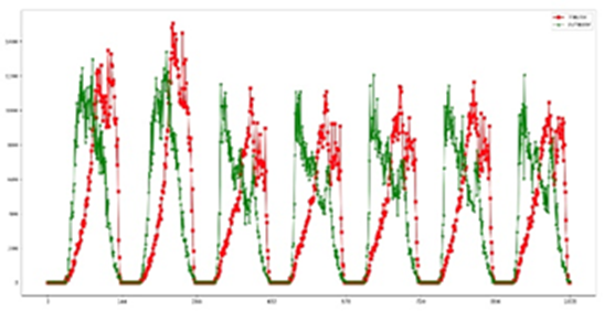
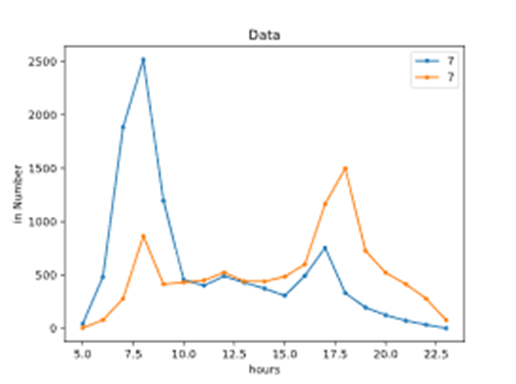
It can be seen from the following figures that the passenger flow of some stations on weekdays is much more than that on weekends, so they can be judged as residential or working. In addition to observing the passenger flow difference between weekends and weekdays, the time distribution of entrances and exits in a day is also noteworthy. It can be seen from the following two figures that some stations have considerable inbound passenger flow in the morning and large outbound passenger flow in the evening, so it is judged that they are working attributes. Some stations are just the opposite (Ni, 2016). If there is a large outbound passenger flow in the morning and a large inbound passenger flow in the evening, it will be judged as a residential property.
(3) Characteristics of station equipment considering the relevant characteristics of card swiping device, the number of equipment at each station has a certain relationship with the passenger flow at the station, and the number of equipment at each period also has a certain relationship with the flow.
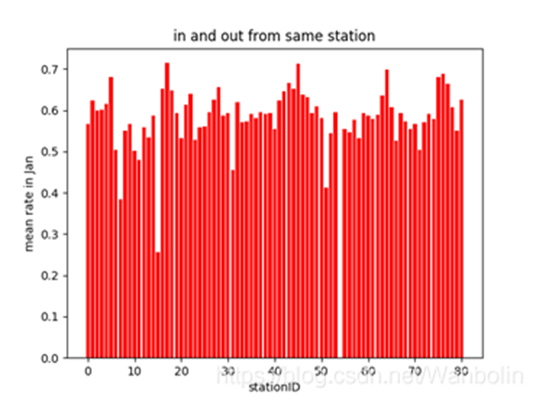
(4) Stable passenger flow
The proportion of people entering and leaving the same station every day in the number of people entering the station. The proportion of passenger flow at each station is relatively stable, some reaching 70%, and the daily fluctuation is relatively regular. It can be considered that most of the people who travel by subway and other public transport live near the subway station. In other words, a large part of the people who go in and out of the same place every day are the same person. This feature is expressed in terms of passenger flow stability.
5.6 summary
In the aspect of feature analysis and feature extraction, we mainly mine features from two angles to distinguish the target and two dimensions, so as to summarize four types of features.
From two aspects, first of all, from the scene, the daily passenger flow changes the same as the previous day, but what causes the fluctuation. Secondly, from the perspective of users, the behavior trajectory of most users should be repeatable, that is, the stability of passenger flow. For the two dimensions, timely distinguish the impact of holidays and peak hours on passenger flow. Spatially, distinguish the impact of passenger flow caused by different geographical locations and different functional attributes. Through the above two angles and dimensions, this paper summarizes four characteristics, namely, basic characteristics, time characteristics, historical time characteristics and geographic information characteristics.
6. Code analysis
6.1 field analysis
The competition data gives 41 field values to predict the daily passenger flow. From the title requirements, we can see that the only prediction result we need to output is "date", "TRADE_ADDRESS" and "predicted passenger flow" data. This means that many of the fields given may be useless. Moreover, we found that the predicted passenger flow is not an intuitive field, so we need to sort it out ourselves. Establish the ipython file Traffic_dataAnalysis. First read the csv data with the pandas Library:
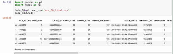
The passenger flow does not appear in the field. According to the requirements of the topic, the daily passenger flow of each site is the sum of transaction types 21 and 22, so the passenger flow is actually the sum of the corresponding lines. Therefore, we choose to use python for drawing to judge the relationship and influence between fields.
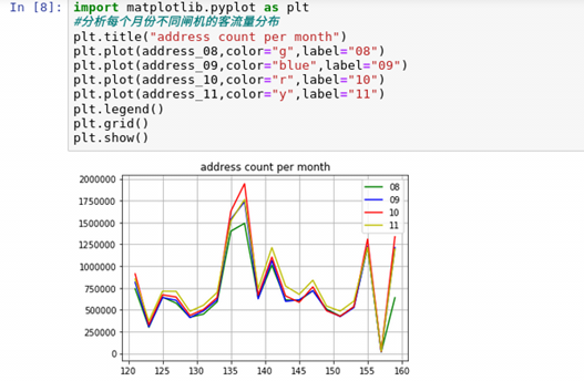
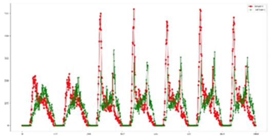
Through the mapping, we can see that the change trend of passenger flow at different card swiping locations every month is very close, so we can know the card swiping location trade_ The data of address field fits very well.
6.2 data cleaning
By analyzing our fields, we conclude that this is a problem about time series model prediction. Other irrelevant attribute fields are not helpful for prediction and can be removed. Because the predicted data unit is day, we first regularize the date, and only take the year, month and day (Y-m-d):
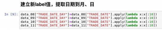
Add field TRADE_DATE_DAY:
Through the sorting and summation of dataframe, we obtain the passenger flow field VAL corresponding to the card swiping location on the corresponding date:
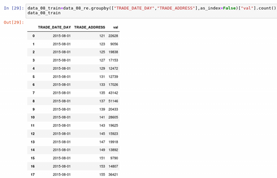
The reorganized data is output, and the data set used to train the time series model is obtained.
6.3 characteristic Engineering
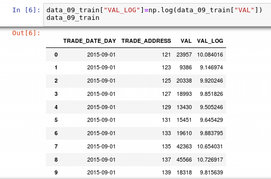
New ipython file Traffic_modelNPre, which operates on the newly output data set. By analyzing the changes of passenger flow in relevant fields, it can be seen that the fluctuation is very large, which is bound to have an impact on the fitting of the model, so we establish a new field VAL_LOG, the VAL is exponentially transformed to make the change value in a relatively small range.
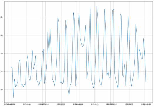
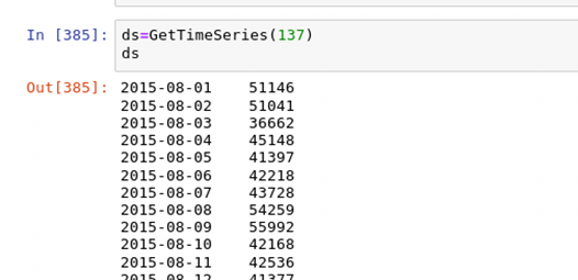
According to the sorted data, it can be analyzed that the time series of subway passenger flow has certain continuity, and the passenger flow in the whole period will be similar in a week. Therefore, we decided to use the time series model as the basic model to solve this problem. At this time, continue to analyze the data:
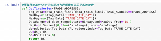
This function can extract the corresponding trade_ Time series data of address and the average number of connections per day.
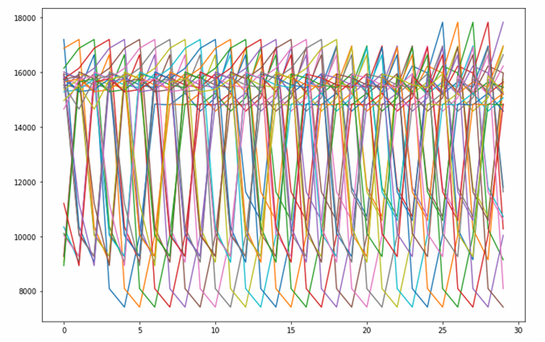
The drawing results are as follows. It can be seen that there are abnormal days.
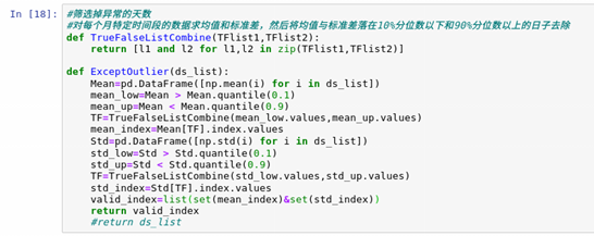
Therefore, it is necessary to write the following function to filter out abnormal days. The filtering strategy here is to calculate the mean and standard deviation of the data of days in a specific time period of each month, and then remove the days when the mean and standard deviation fall below the 10% quantile and above the 90% quantile.
The sequence after removal is as follows:
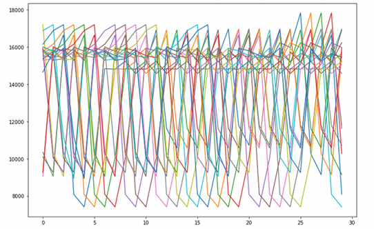
After the abnormal days are filtered out, the data corresponding to the remaining days are retained, and the daily passenger flow corresponding to the abnormal days is taken as the mean of the passenger flow of the normal days of each month, so that the model can be better fitted. In this way, we get a new data set and save it in data_ In the final folder. In this way, the pre work of establishing the model is completed.
6.4 modeling
The data is ready to start building the model. Because the subway pedestrian flow has the characteristics of continuity, we use ARMA to modify the prediction. The model is as follows:
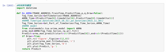
We selected the data from August to October as the temporary training set and the data from November 1 to 7 as the verification set to test the model fitting. Through calculation, the confidence interval of the time series model falls at (2,0), so the values of P and Q of our time series model take 2 and 0 as parameters respectively.
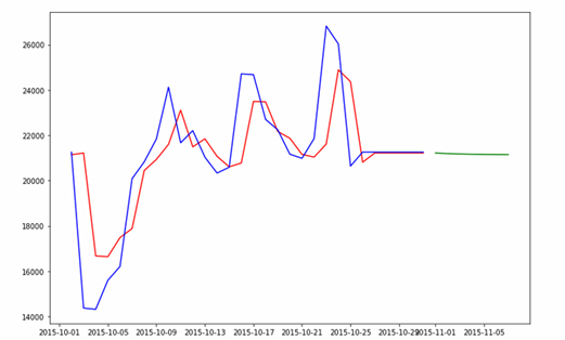
From the result chart, the prediction of time series trend is fairly good, but there are still some deviations. The model is basically built and can be predicted.
6.5 result prediction
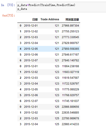
Output to dataframe according to the required tabular form,
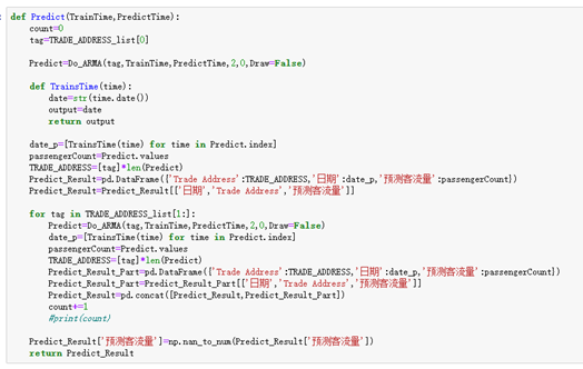
The output completes the prediction data:
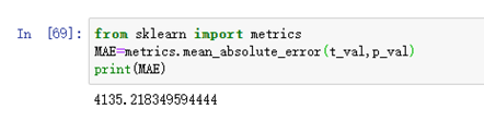
We saved the training model and predicted it with the test set from September 1 to September 7. Compared with the actual data, the final MAE=4135.218.
7. Conclusion
This paper analyzes the complexity and controllability of rail transit passenger flow forecast, analyzes the main error sources of passenger flow forecast in China, and the relevant factors that can be controlled. With more and more attention to urban traffic model in China, the cultivation and growth of traffic model team and the continuous stability of urban planning, it is believed that the accuracy of passenger flow prediction will be higher.
reference
[1] Shi Jinyu, Yang Zeyu, brother Xie Random forest algorithm based on fuzzy decision [J] Computer engineering and design, 2020,41 (08): 2207-2212
[2] Zhou senxin, Li Chao, Wu Decheng Application of Bayesian network in predicting bank credit risk [J] Journal of Jixi University, 2014,14 (10): 42-43 + 63
[3] Wang yuanfan, Shi Yong, Xue Zhi Research on port scanning malicious traffic detection based on decision tree [J] Communication technology, 2020,53 (08): 2002-2005
[4] Li Kai, Tan Haibo, Wang Haiyuan, Xie Yuman, Huang Hongqiao, bu Wenbin, Tan Cong, Peng Xiao, Guo Guang, Liu mouhai, Chen Hao A main network line state detection method, system and medium based on decision tree [P] Hunan Province: cn111612149a, September 1, 2020
[5] Hao Xiaowei, song Haoqi Analysis and Research on financing of small and medium-sized enterprises under Internet finance [J] Economic management abstracts, 2020 (17): 35-36
[6] Chen Shuzhen Optimization of Urban Rail Transit Organization Based on visualization of network passenger flow big data 2019, Vol. 000, No. 4
[7] Song Xiaoyue Research on urban rail transit passenger flow analysis platform based on Spark two thousand and seventeen
[8] An Ju, Chen Feng Research on urban rail transit operation network evaluation technology based on big data two thousand and twenty
[9] Zhong gang Research on passenger travel behavior analysis method of urban comprehensive passenger transport hub based on mobile big data two thousand and nineteen
[10] Xi Yang Research on passenger clustering and passenger flow distribution of Urban Rail Transit Based on AFC data
appendix
Data cleaning
1.	#Days to filter out exceptions
2.	#Calculate the mean and standard deviation of the data in a specific time period of each month, and then remove the days when the mean and standard deviation fall below the 10% quantile and above the 90% quantile
3.	def TrueFalseListCombine(TFlist1,TFlist2):
4.	    return [l1 and l2 for l1,l2 in zip(TFlist1, TFlist2)]
5.	def Exceptoutlier(ds_list):
6.	    Mean=pd . DataFrame( [np.mean(i) for i in ds_list])
7.	    mean_low=Mean > Mean.quantile(0.1)
8.	    mean_up=Mean < Mean. quantile(0.9)
9.	    TF=TrueFalseListcombine(mean_low.values , mean_up.values)
10.	    mean_index=Mean [TF] .index.values
11.	    std=pd.DataFrame([np.std(i) for i in ds_list])
12.	    std_low=std > Std.quantile(0.1)
13.	    std_up=std < std.quantile(0.9)
14.	    TF=TrueFalseListCombine(std_low.values,std_up.values)
15.	    std_index=Std[TF].index.values
16.	    valid_index=list(set(mean_index)&set(std_index))
17.	    return valid_index
18.	    #return ds list
Passenger flow distribution of different gates per month
1.	import matplotlib.pyplot as plt
2.	#Analyze the passenger flow distribution of different gates in each month
3.	plt.title("address count per month")
4.	plt.plot(address_08,color="g",label="08")
5.	plt.plot(address_09,color="blue",label="09")
6.	plt.plot(address_10,color="r",label="10")
7.	plt.plot(address_11,color="y",label="11")
8.	plt.legend()
9.	plt.grid()
10.	plt.show()
Passenger flow distribution on different days of each month
1.	#Analyze the passenger flow distribution on different days of each month
2.	fig=plt.figure(figsize=(12,8))
3.	ax1=fig.add_subplot(2,2,1)
4.	plt.plot(trade_date_08,color="g",label="08")
5.	plt.legend()
6.	ax2=fig.add_subplot(2,2,2)
7.	plt.plot(trade_date_09,color="b",label="09")
8.	plt.legend()
9.	ax3=fig.add_subplot(2,2,3)
10.	plt.plot(trade_date_10,color="r",label="10")
11.	plt.legend()
12.	ax2=fig.add_subplot(2,2,4)
13.	plt.plot(trade_date_11,color="y",label="11")
14.	plt.legend()
15.	plt.show()
Draw a histogram to the weekly passenger flow in different months
1.	#Draw a histogram to the weekly passenger flow in different months
2.	fig=plt.figure(figsize=(12,8))
3.	ax1=fig.add_subplot(2,2,1)
4.	x_data=["Monday","Tuesday","Wednesday","Thursday","Friday","Saturday","Sunday"]
5.	y_data=[data_08_weekday["Monday"],data_08_weekday["Tuesday"],data_08_weekday["Wednesday"],data_08_weekday["Thursday"],data_08_weekday["Friday"],data_08_weekday["Saturday"],data_08_weekday["Sunday"]]
6.	#mapping
7.	plt.bar(x=x_data,height=y_data,label='08',color='r',alpha=.8)
8.	plt.title("Count per week")
9.	plt.legend()
10.	ax2=fig.add_subplot(2,2,2)
11.	x_data=["Monday","Tuesday","Wednesday","Thursday","Friday","Saturday","Sunday"]
12.	y_data=[data_09_weekday["Monday"],data_09_weekday["Tuesday"],data_09_weekday["Wednesday"],data_09_weekday["Thursday"],data_09_weekday["Friday"],data_09_weekday["Saturday"],data_09_weekday["Sunday"]]
13.	#mapping
14.	plt.bar(x=x_data,height=y_data,label='09',alpha=.8)
15.	plt.title("Count per week")
16.	plt.legend()
17.	ax3=fig.add_subplot(2,2,3)
18.	x_data=["Monday","Tuesday","Wednesday","Thursday","Friday","Saturday","Sunday"]
19.	y_data=[data_10_weekday["Monday"],data_10_weekday["Tuesday"],data_10_weekday["Wednesday"],data_10_weekday["Thursday"],data_10_weekday["Friday"],data_10_weekday["Saturday"],data_10_weekday["Sunday"]]
20.	#mapping
21.	plt.bar(x=x_data,height=y_data,label='10',color='g',alpha=.8)
22.	plt.title("Count per week")
23.	plt.legend()
24.	ax4=fig.add_subplot(2,2,4)
25.	x_data=["Monday","Tuesday","Wednesday","Thursday","Friday","Saturday","Sunday"]
26.	y_data=[data_11_weekday["Monday"],data_11_weekday["Tuesday"],data_11_weekday["Wednesday"],data_11_weekday["Thursday"],data_11_weekday["Friday"],data_11_weekday["Saturday"],data_11_weekday["Sunday"]]
27.	#mapping
28.	plt.bar(x=x_data,height=y_data,label='11',color='y',alpha=.8)
29.	plt.title("Count per week")
30.	plt.legend()
31.	plt.show()
Calculate the mean and standard deviation of the data in a specific time period of each month, and then remove the days when the mean and standard deviation fall below the 10% quantile and above the 90% quantile
1.	def TrueFalseListCombine(TFlist1,TFlist2):
2.	    return [l1 and l2 for l1,l2 in zip(TFlist1,TFlist2)]
3.	def ExceptOutlier(ds_list):
4.	    Mean=pd.DataFrame([np.mean(i) for i in ds_list])
5.	    mean_low=Mean > Mean.quantile(0.1)
6.	    mean_up=Mean < Mean.quantile(0.9)
7.	    TF=TrueFalseListCombine(mean_low.values,mean_up.values)
8.	    mean_index=Mean[TF].index.values
9.	    Std=pd.DataFrame([np.std(i) for i in ds_list])
10.	    std_low=Std > Std.quantile(0.1)
11.	    std_up=Std < Std.quantile(0.9)
12.	    TF=TrueFalseListCombine(std_low.values,std_up.values)
13.	    std_index=Std[TF].index.values
14.	    valid_index=list(set(mean_index)&set(std_index))
15.	    return valid_index
16.	    #return ds_list
Forecast in days
1.	import numpy as np
2.	import pandas as pd
3.	def make_mean(c):
4.	    log=c["VAL_LOG"].values
5.	    val=c["VAL"].values
6.	    log_mean=np.mean(log)
7.	    val_mean=np.mean(val)
8.	    return log_mean,val_mean
9.
10.	def loop(c,valid):
11.	    #print(c)
12.	    #print(type(valid[0]))
13.	    log=c["VAL_LOG"].values
14.	    val=c["VAL"].values
15.	    day=c["TRADE_DATE_DAY"]
16.	    add=c["TRADE_ADDRESS"].values
17.	    log_mean,val_mean=make_mean(c)
18.	    time=[]
19.	    all_log=[]
20.	    all_val=[]
21.	    for i in day:
22.	        tmpd=int(i[8:])
23.	        time.append(tmpd)
24.	    Len=len(day)
25.	    for i in range(1,Len+1):
26.	        if(i in valid):
27.	            all_log.append(log[i-1])
28.	            all_val.append(val[i-1])
29.	        else:
30.	            all_log.append(log_mean)
31.	            all_val.append(val_mean)
32.	    frame={
33.	          "TRADE_DATE_DAY":c["TRADE_DATE_DAY"],
34.	         "TRADE_ADDRESS":c["TRADE_ADDRESS"],
35.	        "VAL":all_val,
36.	        "VAL_LOG":all_log
37.
38.
39.	    }
40.	    fram=pd.DataFrame(frame)
41.	    return fram
1.	import pandas as pd
2.	import numpy as np
3.	def Violent():
4.	    t=np.array([pd.datetime(2015,9,1),pd.datetime(2015,11,30)])
5.	    address=[]
6.	    tmp=121
7.	    while(tmp<161):
8.	        address.append(tmp)
9.	        tmp+=2
10.	    #ds_list=DsList(151,Time)
11.	    #ExceptOutlier(ds_list)
12.	    #df_01=data_train[data_train['TRADE_ADDRESS']==151]
13.	    #c=df_01.iloc[ExceptOutlier(ds_list)]
14.	    frame=[]
15.	    for i in address:
16.	        tmp=DsList(i,t)
17.	        df_tmp=data_11_train[data_11_train['TRADE_ADDRESS']==i]
18.	        c=df_tmp.iloc[ExceptOutlier(tmp)]
19.	        #loop(df_tmp,ExceptOutlier(tmp))
20.	        c=loop(df_tmp,ExceptOutlier(tmp))
21.	        #print("_________________________")
22.	        #print(ExceptOutlier(tmp))
23.	        frame.append(c)
24.	    #data_frame=frame[0]
25.	    #del (frame[0])
26.	    valid_day=ExceptOutlier(tmp)
27.	    data_frame=pd.concat(frame,axis=0,ignore_index=True)
28.	    return data_frame
29.	arr=Violent()
30.	arr
time series model
1.	import datetime
2.
3.	def Do_ARMA(TRADE_ADDRESS,TrainTime,PredictTime,p,q,Draw=False):
4.	    Tag_Time_Series=GetTimeSeries(TRADE_ADDRESS)
5.	    ARMA_Time=[PredictTime[0]-timedelta(30),PredictTime[0]-timedelta(1)]
6.	    #ARMA_Time=[pd.datetime(2015,10,31),pd.datetime(2015,11,30)]
7.	    Tag_Time_Series=Get_Part_of_TimeSeries(Tag_Time_Series,ARMA_Time)
8.	    #ARMA model
9.	    from statsmodels.tsa.arima_model import ARMA
10.	    arma_mod=ARMA(Tag_Time_Series,(p,q)).fit()
11.	    Predict=arma_mod.predict(start=str(PredictTime[0]),end=str(PredictTime[1]))
12.	    if Draw==True:
13.	        plt.rc('figure',figsize=(12,8))
14.	        plt.plot(arma_mod.fittedvalues,'r')
15.	        plt.plot(Tag_Time_Series,'b')
16.	        plt.plot(Predict,'g-')
17.	    return Predict
model prediction
1.	  Est_TrainTime = np.array([pd.datetime(2015,month,8),pd.datetime(2016,month,15)])
2.	    Est_PredictTime = np.array([pd.datetime(2015,month,1),pd.datetime(2015,month,7)])
3.	    y = Get_Part_of_TimeSeries(GetTimeSeries(TRADE_ADDRESS_List[i]),Est_PredictTime)
4.	    prey0 =Imitate1(TRADE_ADDRESS_List[i],Est_TrainTime,Est_PredictTime)
5.	    prey1 =Imitate2(TRADE_ADDRESS_List[i],Est_TrainTime,Est_PredictTime)
6.	    prey2=Do_ARMA(TRADE_ADDRESS_List[i],Est_TrainTime,Est_PredictTime,0,1)
7.	    prey3 = Combine(TRADE_ADDRESS_List[i],Est_TrainTime,Est_PredictTime,Ratio_Dict)
8.	    y.plot()
9.	    prey0.plot()
10.	    prey1.plot()
11.	    prey2.plot()
12.	    prey3.plot()
13.	    plt.legend(['real','imitate1','imitate2','arma','combine'])
14.	    title = ('2015-'+str(month))
15.	    plt.title(title)[0]
Welcome to join me for wechat learning and discussion