preface
Performance tuning of Java virtual machine is a very broad topic and a very difficult process in practice. Because it needs a systematic optimization method and clear optimization expectations. The default JVM parameters attempt to provide acceptable performance in most cases; However, depending on the behavior of the application and the workload it is in, the default values may not produce the desired results. If the Java virtual machine does not run as expected, you may need to benchmark and tune your application to find an appropriate set of JVM parameters.
In most cases, "JVM tuning" is about "Java GC tuning". The first topic about HotSpot virtual machine in the official JAVA manual is the HotSpot Virtual Machine Garbage Collection Tuning Guide.
This paper records a "basic step and process" summarized from the GC tuning of real business development. Combined with some reference materials, this paper gives a case and personal understanding of this knowledge point.
1. Preparation before optimization
- Deeply understand the business logic that needs to be optimized
- In depth understanding of Java virtual machine related concepts (books, official documents)
- Think about the purpose of JVM tuning. Do you really need tuning? More than 90% of the problems are caused by business code. Can we achieve better results by focusing on the optimization of business logic?
There are some factors that affect the final tuning parameters you get:
- Version of JDK
- Server hardware
- operating system
- Load curve of system
- The business type of the system, and the optimization needs to focus on the business type
- Data set of the system
All of the above constitutes an environment for tuning GC performance. The more specific the tuning parameters are, the less generic the solution will be and the less applicable the environment will be. This means that if any variables change (for example, more users are granted permission to request applications, application upgrades, hardware upgrades), any performance tuning you make may need to be reassessed.
In addition, it must be understood that explicit tuning may actually reduce performance. It is important to continuously monitor the application and check that the tuning based assumptions are still valid. If you still fail to achieve your goal after careful debugging, you may want to consider changes other than GC tuning, such as replacing more appropriate hardware, operating system tuning, and application tuning.
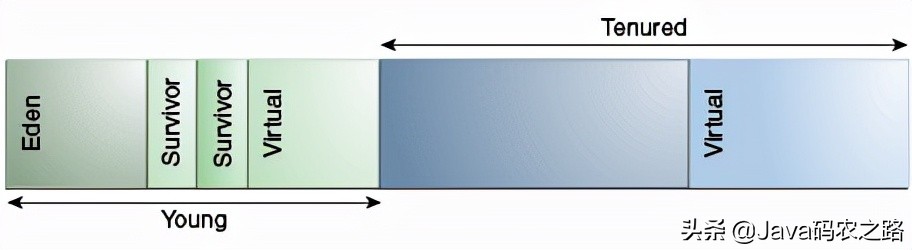
Default Arrangement of Generations . The picture is not important. Look at the text~
2. Select optimization objectives
JVM optimization first needs to select the target. Set values around these goals when preparing the system for GC tuning in the next step. Referential target selection direction:
- Latency - the Stop The World (STW) caused by the JVM when performing garbage collection. There are two main indicators, average GC latency and maximum GC latency. The motivation for this goal is usually related to the customer's perceived performance or responsiveness.
- Throughput - the percentage of time that the JVM is available to execute the application. The more time available to execute the application, the more processing time available to service requests. It should be noted that high throughput and low latency are not necessarily related - high throughput may be accompanied by long but infrequent pauses.
- Memory cost - memory footprint is the amount of memory consumed by the JVM to execute the application. If the application environment has limited memory, setting this as a target can also reduce costs.
The above contents can be found in the HotSpot tuning section of the official Java manual, and some empirical optimization principles are as follows:
- MinorGC is preferred. In most applications, most of the garbage is created by the recent transient object allocation, so the younger generation of GC is preferred. The shorter the life cycle of young generation objects, the objects with short survival time will not be assigned to the old age due to factors such as dynamic age judgment and spatial allocation guarantee; At the same time, the longer the object life cycle in the old age, the more efficient the overall garbage collection of the JVM, which will lead to higher throughput.
- Set the appropriate heap size. The more memory you give the JVM, the lower the collection frequency. In addition, this also means that the size of the younger generation can be appropriately adjusted to better cope with the creation speed of short-term objects, which reduces the number of objects allocated to the older generation.
- Set simple goals. In order to make things easier, set the JVM tuning goal a little simpler. For example, select only two of the performance goals to adjust at the expense of the other or even only one. Usually, these goals compete with each other. For example, in order to improve throughput, the more memory you give to the heap, the longer the average pause time may be; Conversely, if you give less memory to the heap and reduce the average pause time, the pause frequency may increase and reduce the throughput. Similarly, for the size of the heap, if the size of all generational regions is appropriate, it can provide better latency and throughput, which is usually at the expense of JVM occupancy.
In short, adjusting GC is a balanced behavior. Usually, you can't achieve all the goals just by adjusting GC.
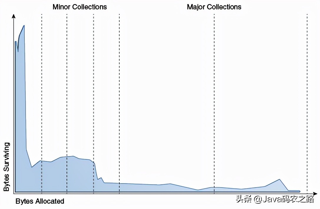
Typical Distribution for Lifetimes of Objects . The picture is not important. Look at the text~
3. Business logic analysis
Here, the real business system is not taken out for analysis, but a similar scenario is simulated. The general business information is as follows:
- A microservice system (in this case, a SpringBoot Demo, hereinafter referred to as D Service) mainly provides caching and search services for book entity information
- The underlying database is MySQL+Redis+Elasticsearch
- The business scenario is to provide cache and book information retrieval to other micro service modules or other parts
- MySQL+Redis + application memory multi-level cache is used in the actual implementation of requirements
In terms of the nature of D service, it is not a back-end service with strong user interaction. It is mainly aimed at other micro services in the Department and back-end services in other departments, Therefore, the response speed (latency) of requests does not belong to the first goal, so the main tuning goal can be set to increase throughput or reduce memory consumption. Of course, since the service itself is not bloated and production resources are not very tight, reducing memory is not considered, so the final goal is to increase throughput.
From the perspective of business logic, it mainly refers to the addition, deletion, modification and query of book information. More than 90% of the request traffic is query, and the addition, deletion and modification are mostly the maintenance of multi-party data within the service.
There are many types of queries. From the perspective of objects, most of them are short-term objects, such as:
- Complex ES query statement objects generated through the advanced search (AS) module (small amount of data, medium frequency and very short survival time)
- Data response objects that integrate business logic from multiple data sources (in the amount of data, the frequency is very high and the survival time is very short)
- Data objects temporarily stored in memory in multi-level cache system (small amount of data, high frequency and medium survival time, because it is LRU cache)
- Regularly maintain the data objects distributed by task processing (large amount of data, low frequency and very short survival time)
The only business objects that may enter the old age are those in the memory cache. This block is often kept within hundreds of MB in combination with the business volume + expiration time. The size here is the result of Dump heap memory + MAT analysis in multiple pressure tests.
Combining all the above information, we can see that this is an application in which most objects will not survive for too long. Therefore, the preliminary idea is to increase the size of the young generation, so that most objects can be recycled in the young generation and reduce the probability of entering the old age.
The Demo code is posted below. In order to simulate a similar situation, the code in the Demo may adopt some tricks or extreme settings, which may not well express the original logic, but a Demo that can run in less than 40 lines is easier to understand than a complex project or open source software
Copy code 1234567891011213141516171819202122232425262728293033132334353637383940414243444546 JAVA/**
 * @author fengxiao
 * @date 2021-11-09
 */
@RestController
@SpringBootApplication
public class Application {
    private final Logger logger = LoggerFactory.getLogger(Application.class);

    //1. Simulate memory cache, short-term object
    private Cache<Integer, Book> shortCache;

    //2. Simulate the medium survival time objects in the business process, so that the short-term objects are more likely to enter the old generation
    private Cache<Integer, Book> mediumCache;

    public static void main(String[] args) {
        SpringApplication.run(Application.class, args);
    }

    @PostConstruct
    public void init() {
        //3. The value setting of local cache here is not referential in the actual business, but tries to make some objects enter the old generation under the initial setting
        shortCache = Caffeine.newBuilder().maximumSize(800).initialCapacity(800)
                .expireAfterWrite(3, TimeUnit.SECONDS)
                .removalListener((k, v, c) -> logger.info("Cache Removed,K:{}, V:{}, Cause:{}", k, v, c))
                .build();
        mediumCache = Caffeine.newBuilder().maximumSize(1000).softValues()
                .expireAfterWrite(30, TimeUnit.SECONDS)
                .build();
    }

    @GetMapping("/book")
    public Book book() {
        //4. Simulate the consumption of short-term object generation of other modules in the business processing process. This parameter can be adjusted to increase the frequency of YoungGC without interference to the elderly generation
//        byte[] bytes = new byte[16 * 1024];
        return shortCache.get(new Random().nextInt(5000), (id) -> {
                    //5. Simulate normal LRU cache scenario consumption
                    Book book = new Book().setId(id).setArchives(new byte[256 * 1024]);
                    //6. Simulate the normal consumption of the old age in the business system
                    mediumCache.put(id, new Book().setArchives(new byte[128 * 1024]));
                    return book;
                }
        );
    }
}
4. Prepare the tuning environment
Once the direction is determined, you need to prepare the environment for GC tuning. The result of this step will be the value of your chosen goal. In short, goals and values will become the system requirements of the environment to be tuned.
4.1 container image selection
In fact, it is to select the JDK version. Different versions of JDK have different combinations of collectors, and it is also very important to select collectors according to business types.
Because the JDK version used in daily work is still 1.8, PS/PO (also the default collector of JDK1.8 server) is naturally selected in combination with the throughput target mentioned above. The characteristics and combination of collectors are not expanded here. You need to consult books and documents by yourself.
4.2 start / warm up the workload
Before measuring the GC performance of a particular application JVM, you need to be able to get the application to work and reach a steady state. This is achieved by applying load to the application.
It is recommended to model the load as a steady-state load that you want to tune GC, that is, a load that reflects the usage pattern and usage of the application when it is used in the production environment. Here, you can pull up colleagues from the testing department to complete it together, and make the target program close to the state in real production by means of pressure measurement and flow playback. At the same time, you should pay attention to similar hardware, operating system version, loading configuration file, etc. Load environment and quota can be easily realized through containerization.
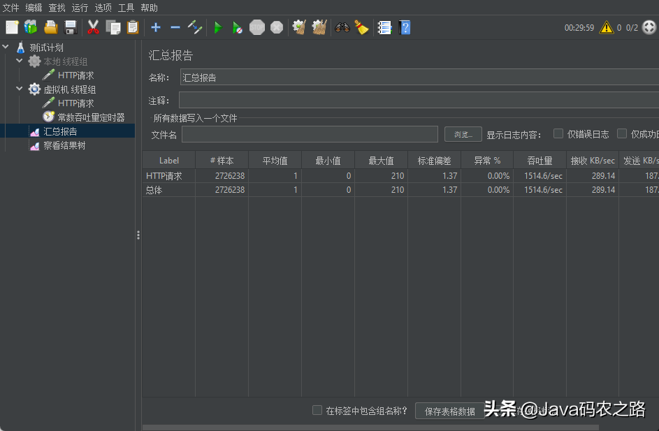
Demo here, MeterSphere is used to simulate the pressure. Simply, you can also use Jmeter to quickly start or directly record the real traffic for playback.
4.3 enable GC log / monitoring
It is believed that most production systems are enabled by default. If JDK9 is the following:
Copy code 1 SHELLJAVA_OPT="${JAVA_OPT} -Xloggc:${BASE_DIR}/logs/server_gc.log -verbose:gc -XX:+PrintGCDetails -XX:+PrintGCDateStamps -XX:+PrintGCTimeStamps -XX:+UseGCLogFileRotation -XX:NumberOfGCLogFiles=10 -XX:GCLogFileSize=100M"
JDK9 is integrated into xlog parameters:
Copy code 1 SHELL-Xlog:gc*:file=${BASE_DIR}/logs/server_gc.log:time,tags:filecount=10,filesize=102400"
Then you need to understand the meaning of various fields in the GC log. Here, it is recommended to observe more GC logs in your system to understand the meaning of the log.
As for monitoring, you can access a monitoring system like Prometheus+Grafana to monitor + alarm. No one wants to stare at the GC log every day. Therefore, a Prometheus+Grafana monitoring is temporarily set up here to facilitate the display of results, and Elasticsearch+Kibana is used to analyze GC logs. Start Grafana with minimal configuration:
Copy code 123456789101121314151617 YAMLversion: '3.1'

services:
  prometheus:
    image: prom/prometheus
    volumes:
      - ./prometheus/prometheus.yml:/etc/prometheus/prometheus.yml
    ports:
      - 9090:9090
    container_name: prometheus
  grafana:
    image: grafana/grafana
    depends_on:
      - prometheus
    ports:
      - 3000:3000
    container_name: grafana
After making some basic configurations for Prometheus and Grafana, you can import a JVM related monitoring panel at will:
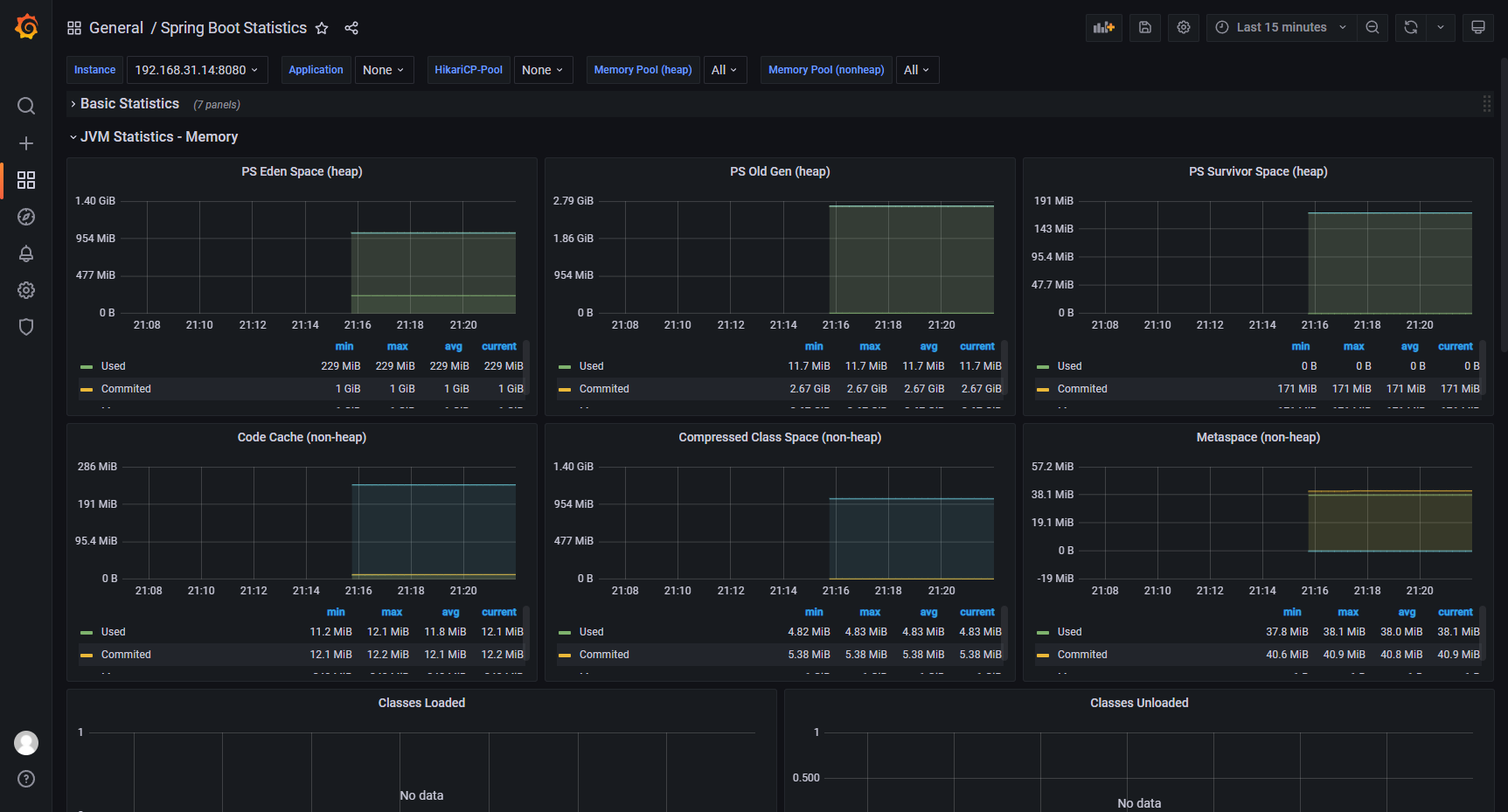
4.4 determining memory footprint
Memory footprint refers to the amount of main memory used or referenced by a program at runtime (Wiki portal: memory footprint, hereinafter referred to as memory footprint)
In order to optimize the size of the JVM generation, you need to know the size of the steady-state active dataset well. You can obtain relevant information in the following two ways:
- Observe from GC log
- Observation from visual monitoring (intuitive)
5. Determine system requirements
Returning to performance goals, we discussed three performance goals for VM GC tuning. Now you need to determine the values of these goals, which represent the system requirements of the environment in which you are tuning GC performance. Some system requirements to be determined are:
- Acceptable average Minor GC pause time
- Acceptable average GC pause time
- Maximum tolerable Full GC pause time
- Minimum acceptable throughput in percent of available time
Generally, if you focus on Latency or Footprint targets, you may prefer a smaller heap memory value and use a smaller throughput value to set the maximum tolerance of pause time; Conversely, if you focus on throughput, you may want to use a larger pause time value and a larger throughput value without a maximum tolerance.
It is better to evaluate and formulate this part in combination with the current situation of the business system in charge, and optimize it on a benchmark value. Take the original throughput of D service as an example (various complex situations in the actual business system should be carefully considered):
| system requirements | value |
| Acceptable Minor GC pause time: | 0.2 seconds |
| Acceptable Full GC pause time: | 2 seconds |
| Minimum acceptable throughput: | 95% |
In this step, you can understand the behavior based tuning in the official Java documents and some ready-made JVM tuning cases. The important thing is to understand the ideas and determine the requirements in combination with your own business.
6. Set sample parameters and start pressure measurement
The following are the benchmark operating parameters of service D in this example
Copy code 12345678910111213 SHELLjava -Xms4g -Xmx4g
-XX:-OmitStackTraceInFastThrow
-XX:+HeapDumpOnOutOfMemoryError
-XX:HeapDumpPath=logs/java_heapdump.hprof
-Xloggc:logs/server_gc.log
-verbose:gc
-XX:+PrintGCDetails
-XX:+PrintGCDateStamps
-XX:+PrintGCTimeStamps
-XX:+UseGCLogFileRotation
-XX:NumberOfGCLogFiles=10
-XX:GCLogFileSize=100M
-jar spring-lite-1.0.0.jar
At this time, the jmap command is used to analyze the heap area as follows. The program runs in the virtual machine. It is found that GC is frequent in some cases when debugging parameters, so only four logical processors are allocated:
Copy code 12345678910112131415161718192021222324252627282930331323343536373839404142434445 SHELLDebugger attached successfully.
Server compiler detected.
JVM version is 25.40-b25

using thread-local object allocation.
Parallel GC with 4 thread(s)

Heap Configuration:
   MinHeapFreeRatio         = 0
   MaxHeapFreeRatio         = 100
   MaxHeapSize              = 4294967296 (4096.0MB)
   NewSize                  = 1431306240 (1365.0MB)
   MaxNewSize               = 1431306240 (1365.0MB)
   OldSize                  = 2863661056 (2731.0MB)
   NewRatio                 = 2
   SurvivorRatio            = 8
   MetaspaceSize            = 21807104 (20.796875MB)
   CompressedClassSpaceSize = 1073741824 (1024.0MB)
   MaxMetaspaceSize         = 17592186044415 MB
   G1HeapRegionSize         = 0 (0.0MB)

Heap Usage:
PS Young Generation
Eden Space:
   capacity = 1073741824 (1024.0MB)
   used     = 257701336 (245.76314544677734MB)
   free     = 816040488 (778.2368545532227MB)
   24.00030717253685% used
From Space:
   capacity = 178782208 (170.5MB)
   used     = 0 (0.0MB)
   free     = 178782208 (170.5MB)
   0.0% used
To Space:
   capacity = 178782208 (170.5MB)
   used     = 0 (0.0MB)
   free     = 178782208 (170.5MB)
   0.0% used
PS Old Generation
   capacity = 2863661056 (2731.0MB)
   used     = 12164632 (11.601097106933594MB)
   free     = 2851496424 (2719.3989028930664MB)
   0.42479301014037324% used

14856 interned Strings occupying 1288376 bytes.
The Jmeter request settings are as follows. Because there is no business logic in the Demo process, even if a single thread has a high throughput, pay attention to the differences in the test environment configuration. For example, if I directly use Jmeter in the IDE, the single thread throughput can reach 1800/s, while in a virtual machine with a low configuration, multiple threads are required to achieve a similar throughput level, Therefore, several threads can be added and the throughput timer can be used to control the request rate at the same time:
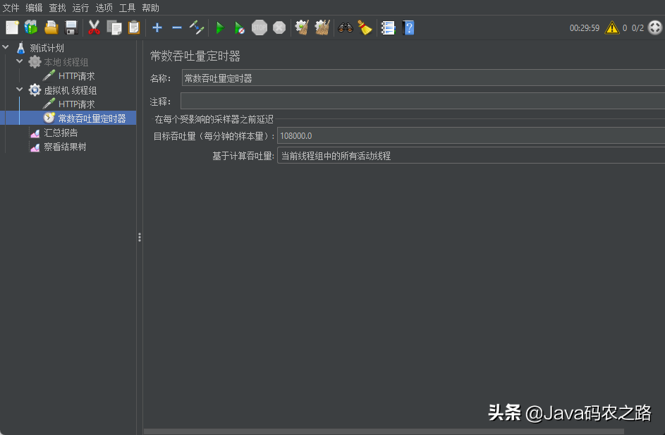
Make repeated requests for adjusting parameters for half an hour each time. This is for the Demo. If the real business system takes more time to sample
7. Analyze GC logs
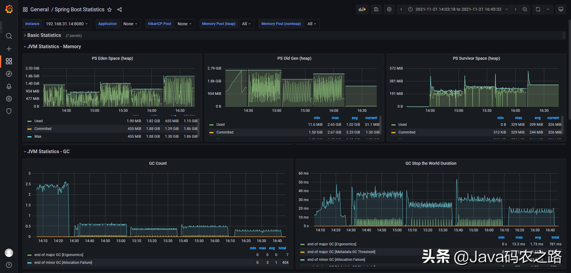
For the Demo in this example, the GC log results under four parameters are taken. The overview of Grafana is as follows:
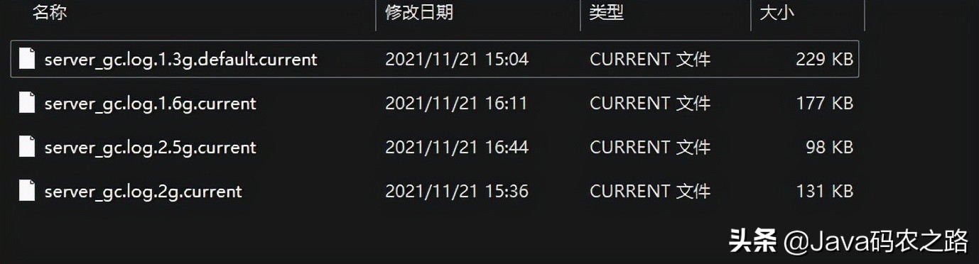
Finally, four GC log samples are generated. The memory size in the file name refers to the size of the younger generation. For production services, more parameter samples can be collected from multiple angles:
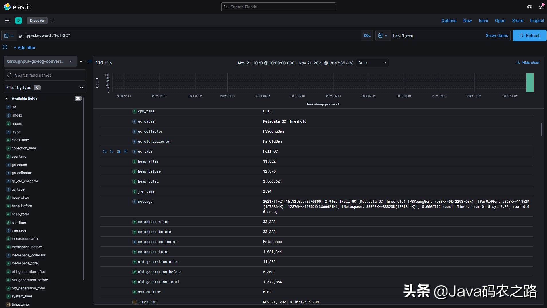
7.1 import Elasticsearch
Next, we import the GC log into Elasticsearch and check it in Kibana (note that Elasticsearch and Kibana must be above version 7.14, otherwise subsequent operations cannot be completed due to version):
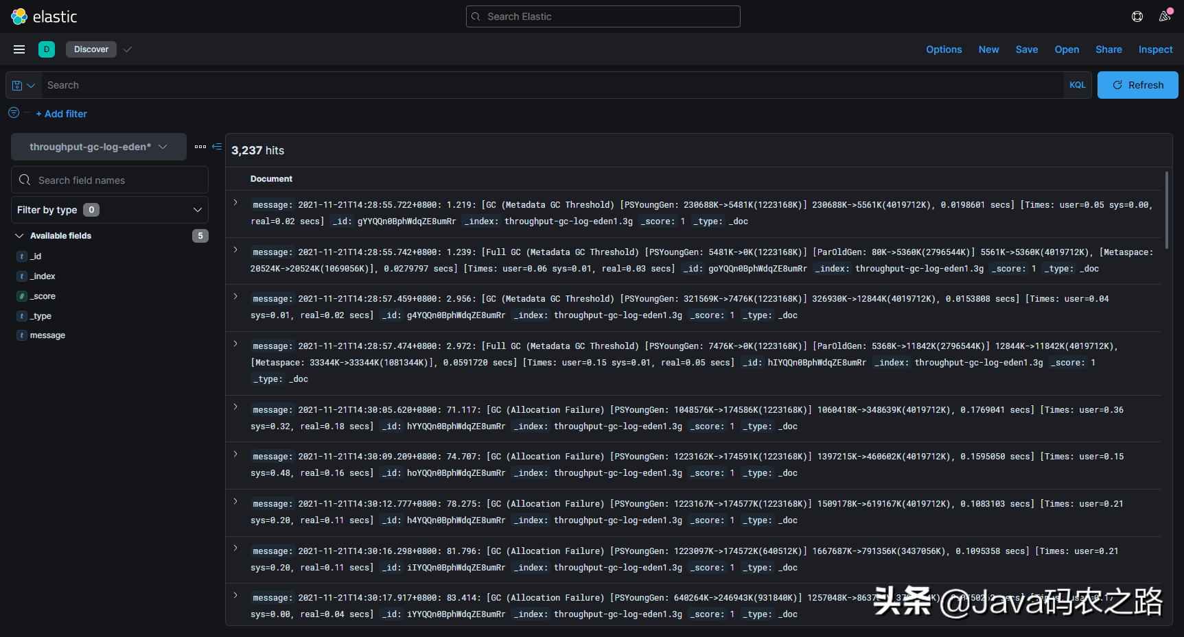
At this time, the GC in the index is still in the original format, just like opening it directly in Linux, so we need to split the log into key fields through Grok Pattern. The actual development scenario can be parsed and transmitted with Logstash. This is just a demonstration, so the index data can be processed quickly through IngestPipeline + Reindex.
After success, the index is as follows. We have structured GC data that can make visual panels (Grok Pattern will not be shared here, mainly because the expression I spent half an hour writing can not perfectly match some special GC log lines = =. It is also recommended that you write matching expressions yourself, so that you can carefully digest the structure of GC logs)
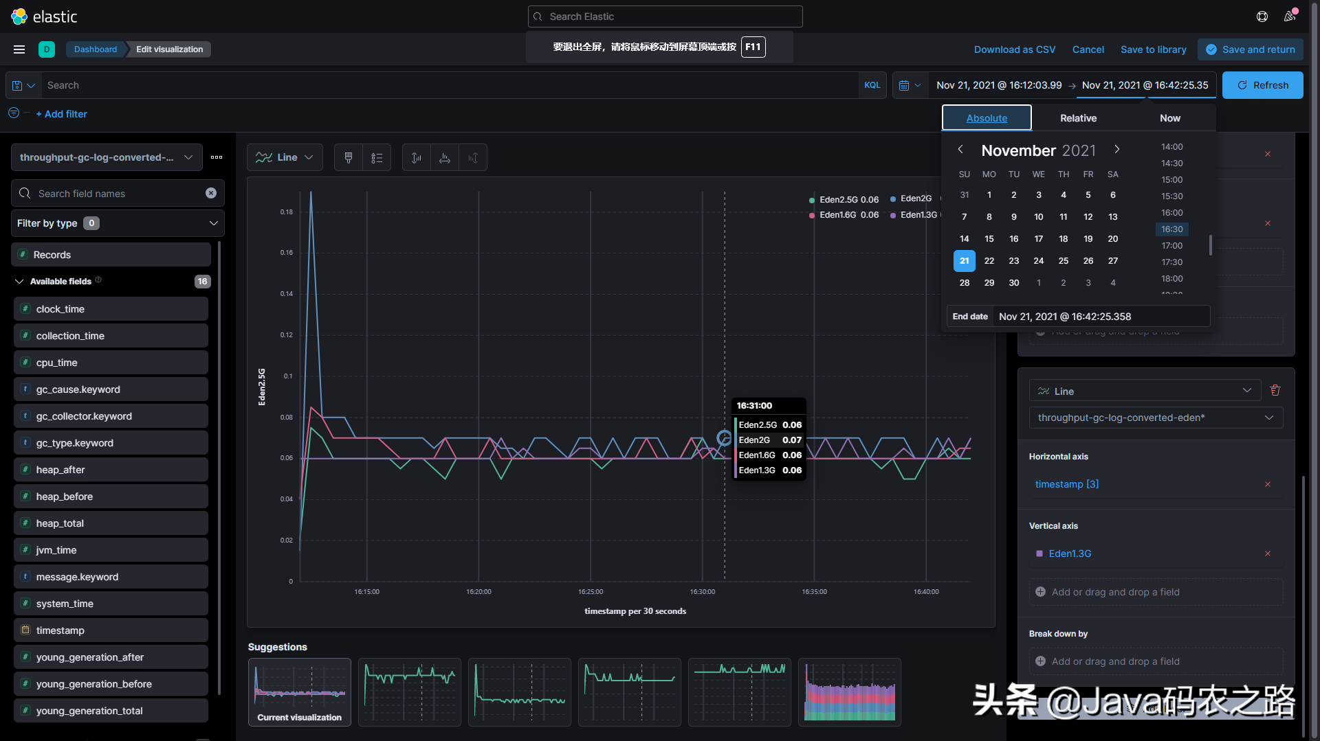
7.2 making visual panel
Now find the start time and end time corresponding to each log index through aggregation
Copy code 12345678910112131415161718192021222324252627282930331323343536373839404142434445464748495051525354 JSONGET throughput-gc-log-converted*/_search
{
  "size": 0,
  "aggs": {
    "index": {
      "terms": { "field": "_index", "size": 10 },
      "aggs": {
        "start_time": {
          "min": { "field": "timestamp" }
        },
        "stop_time": {
          "max": { "field": "timestamp" }
        }
      }
    }
  }
}
// The response is as follows:
"aggregations" : {
    "index" : {
      "doc_count_error_upper_bound" : 0,
      "sum_other_doc_count" : 0,
      "buckets" : [
        {
          "key" : "throughput-gc-log-converted-eden1.3g",
          "doc_count" : 1165,
          "start_time" : { "value" : 1.637476135722E12, "value_as_string" : "2021-11-21T06:28:55.722Z"
          },
          "stop_time" : { "value" : 1.637478206592E12, "value_as_string" : "2021-11-21T07:03:26.592Z" }
        },
        {
          "key" : "throughput-gc-log-converted-eden1.6g",
          "doc_count" : 898,
          "start_time" : { "value" : 1.637480290228E12, "value_as_string" : "2021-11-21T07:38:10.228Z"
          },
          "stop_time" : { "value" : 1.637482100695E12, "value_as_string" : "2021-11-21T08:08:20.695Z" }
        },
        {
          "key" : "throughput-gc-log-converted-eden2.0g",
          "doc_count" : 669,
          "start_time" : { "value" : 1.63747831467E12, "value_as_string" : "2021-11-21T07:05:14.670Z"
          },
          "stop_time" : { "value" : 1.637480148437E12, "value_as_string" : "2021-11-21T07:35:48.437Z" }
        },
        {
          "key" : "throughput-gc-log-converted-eden2.5g",
          "doc_count" : 505,
          "start_time" : { "value" : 1.637482323999E12, "value_as_string" : "2021-11-21T08:12:03.999Z"
          },
          "stop_time" : { "value" : 1.637484145358E12, "value_as_string" : "2021-11-21T08:42:25.358Z" }
        }
      ]
    }
  }
After determining the time range, enter the Dashboard page and create a visual panel as follows. The reason why we need a precise time range is that we need a precise offset time to compare the performance of GC under different conditions. Now we can observe the GC times and GC time-consuming under different settings. In addition, it is better to have ready-made icons when sharing or reporting the tuning results to colleagues or leaders than a pile of data~
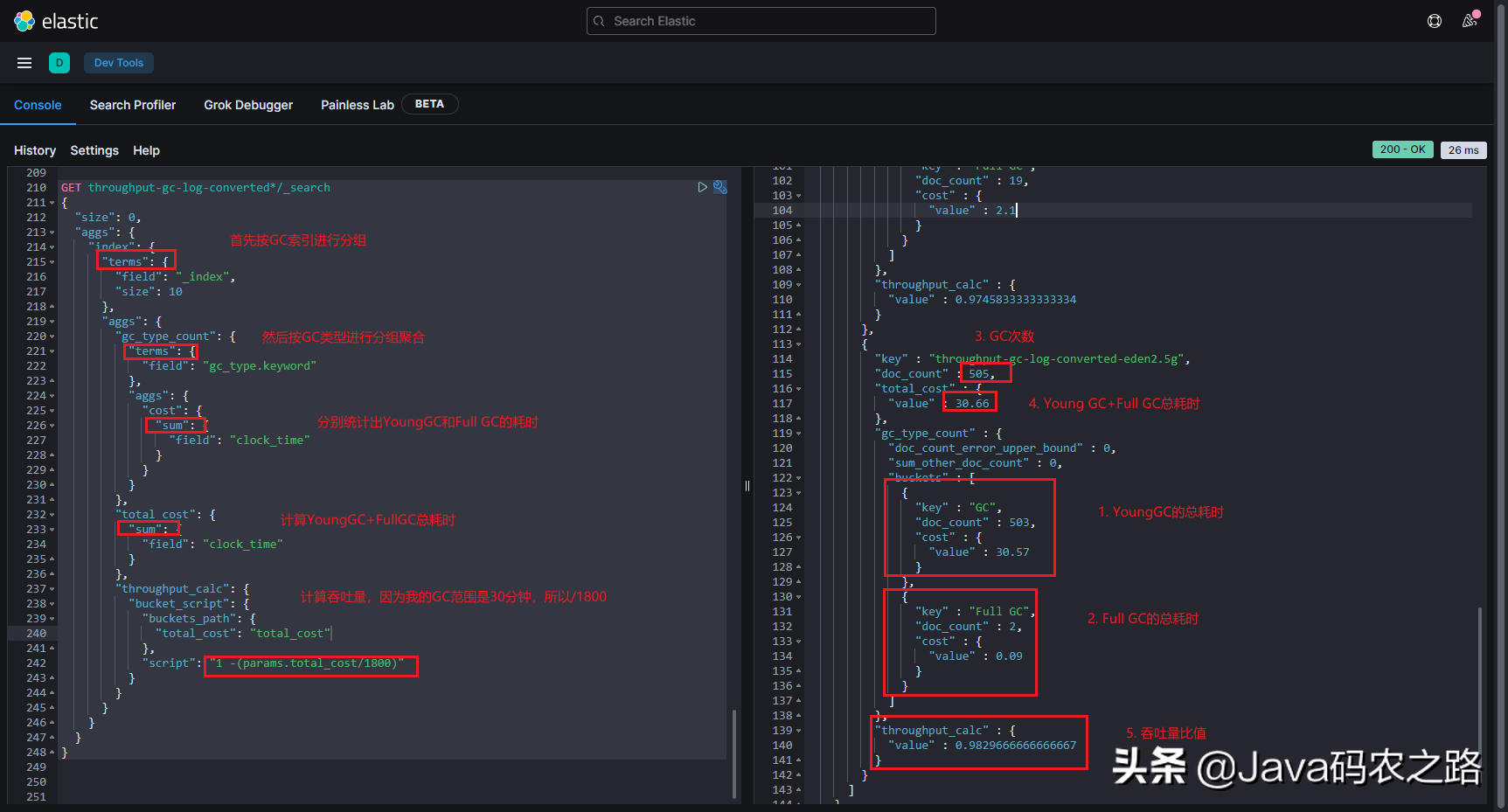
7.3 obtaining performance indicators
Use aggregate statements to calculate GC indicators:
Copy code 1234567891011213141516171819202122232425262728293031 JSGET throughput-gc-log-converted*/_search
{
  "size": 0,
  "aggs": {
    "index": {
      "terms": {
        "field": "_index",
        "size": 10
      },
      "aggs": {
        "gc_type_count": {
          "terms": { "field": "gc_type.keyword" },
          "aggs": {
            "cost": {
              "sum": { "field": "clock_time" }
            }
          }
        },
        "total_cost": {
          "sum": { "field": "clock_time" }
        },
        "throughput_calc": {
          "bucket_script": {
            "buckets_path": { "total_cost": "total_cost" },
            "script": "1 -(params.total_cost/1800)"
          }
        }
      }
    }
  }
}
The results are shown in the figure:
8. Determine the result parameters
The results after analysis are not important, because the final decision depends on the tuner's understanding of the business system and garbage collection. In the previous section, we obtained the throughput performance of D Service under different parameters. Whether to choose the parameter with the best value should be combined with other situations.
In this example, 98.2% of the best throughput results are obtained under the 2.5G setting of the younger generation. Why not try to increase the size of the younger generation? Because it is meaningless, it is unlikely that the ratio of young generation to old generation will exceed 3:1 in a real business system. Even if there is, it seems that such virtual machine parameters are a little extreme. Will the business requirements never change?
Finally, some mature and stable tuning criteria and experience must be combined with how to change parameters. For example, you can see in various GC optimization blogs, such as:
- The maximum heap size should be between 3 - 4 times the average of older generations.
- Observe the memory footprint. The elderly generation should not be less than 1.5 times the average value of the elderly generation.
- The younger generation should be greater than 10% of the whole heap.
- When resizing the JVM, do not exceed the amount of physical memory available.
- . . . . .
Returning to the Demo in this example, if I see a comprehensive result of production service, I will not explicitly set - Xmn to any value, but set a relative ratio such as - XX:NewRatio=1 (this article refers to the latest real production service tuning, and the real optimization result is NewRatio and some other values).
If you carefully observe the Demo code and analyze its object consumption while reading the article, you will find that the author spent a lot of time modulating some parameters to make the Demo under the lower allocation of the younger generation, and the objects of the younger generation will enter the dying state as soon as they enter the older generation, resulting in high-frequency GC; When the younger generation reached the threshold of 2.3G +, the cache object and timeout reached a delicate balance. It is impossible for the cache object to enter the older generation and will not produce Full GC. As shown in the following aggregation results (this SpringBoot program startup foundation generates two full GCS):
Copy code 1234567891011213141516171819202122232425262728293033132335363738394041424344454647484950515253545556575758590616263646566 JSON{
    "key": "throughput-gc-log-converted-eden1.3g",
    "doc_count": 1165,
    "total_cost": { "value": 75.87 },
    "gc_type_count": {
        "doc_count_error_upper_bound": 0,
        "sum_other_doc_count": 0,
        "buckets": [
            {
                "key": "GC",
                "doc_count": 1113,
                "cost": { "value": 69.86 }
            },
            {
                "key": "Full GC",
                "doc_count": 52,
                "cost": { "value": 6.01 }
            }
        ]
    },
    "throughput_calc": { "value": 0.95785 }
},
{
    "key": "throughput-gc-log-converted-eden2.0g",
    "doc_count": 669,
    "total_cost": { "value": 45.75 },
    "gc_type_count": {
        "doc_count_error_upper_bound": 0,
        "sum_other_doc_count": 0,
        "buckets": [
            {
                "key": "GC",
                "doc_count": 650,
                "cost": { "value": 43.65 }
            },
            {
                "key": "Full GC",
                "doc_count": 19,
                "cost": { "value": 2.1 }
            }
        ]
    },
    "throughput_calc": { "value": 0.9745833333333334 }
},
{
    "key": "throughput-gc-log-converted-eden2.5g",
    "doc_count": 505,
    "total_cost": { "value": 30.66 },
    "gc_type_count": {
        "doc_count_error_upper_bound": 0,
        "sum_other_doc_count": 0,
        "buckets": [
            {
                "key": "GC",
                "doc_count": 503,
                "cost": { "value": 30.57 }
            },
            {
                "key": "Full GC",
                "doc_count": 2,
                "cost": { "value": 0.09 }
            }
        ]
    },
    "throughput_calc": { "value": 0.9829666666666667 }
}
Such a coincidence rarely occurs in the actual fast iterative production service. Even if it does occur, don't make smart choices. Because on the complex business system, any simple change of business requirements can easily destroy the carefully set parameters. Of course, it doesn't matter if your system is a middleware product or similar software released regularly.
9. Condition after change of measurement parameters
This step usually takes longer than the tuning process. After the tuning direction and parameters are actually determined, the results are expected and connected with the colleagues in the testing department. All aspects of testing are started, and the index changes are collected from the top level of the system. If successful, it will take several weeks. Maybe the parameter configuration can be merged into the trunk branch of the configuration warehouse.
If the result doesn't meet expectations, start again~
10. Summary
There are a lot of miscellaneous things recently. I hurriedly sorted out an essay. The structure and wording may not have been carefully sorted out. Please understand=_=