Supervised algorithm KNN/K nearest neighbor
1: Principle
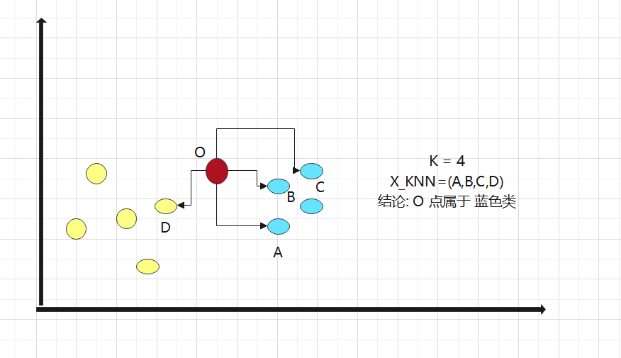
1. Calculate the Euclidean distance from o point to all points
Oh
Surname
distance
leave
:
d
=
(
x
a
−
x
b
)
2
+
(
y
a
−
y
b
)
2
Euclidean distance: d = \sqrt{(x_a-x_b)^2+(y_a-y_b)^2}
Euclidean distance: d=(xa − xb) 2+(ya − yb) 2
2. Assuming K = 4, select the K points with the smallest distance
3. What categories do K points belong to
4. Find the maximum number of classes in K points, then divide point O into this class
2: The advantages and disadvantages of the algorithm are extremely variable
2.1 advantages and disadvantages
The value of algorithm parameter K affects the effect of the model, so the value of K needs to be determined through the learning curve
Note: the parameters passed artificially are called super parameters, so the parameter adjustment of the model generally refers to the adjustment of super parameters
1. When the K value is larger, the deviation is larger, and under fitting may occur
2. When the K value is smaller, the variance is larger, and over fitting may occur
2.2 algorithm variants
Reason: the value of K may cause the same number of classes, which makes it impossible to classify (because the weight of each point is the same by default)
Variant 1: specify different distance weights for different neighbors. For example, the closer the distance, the greater the weight
Implementation: by specifying the weights parameter in the algorithm
Variant 2: use points within a certain radius to replace the nearest K points
In scikit learn, the RadiusNeighborsClassifier implements a variant of this algorithm
The algorithm is more suitable for the case of uneven data sampling
3: Implementation of KNN Algorithm in python
#All lines can be output
from IPython.core.interactiveshell import InteractiveShell
InteractiveShell.ast_node_interactivity = "all"
import numpy as np
import pandas as pd
import matplotlib.pyplot as plt
# Solve the confusion of negative sign of coordinate axis scale
plt.rcParams['axes.unicode_minus'] = False
# Solve the problem of Chinese garbled code
plt.rcParams['font.sans-serif'] = ['Simhei']
plt.style.use('ggplot')

#Building data sets
data1 = {
    'height':[170,189,178,165,166,160,156,158,160,155],
    'weight':[110,120,126,112,108,100,98,95,110,85],
    'Gender':[1,1,1,1,1,0,0,0,0,0]
}
data = pd.DataFrame(
    data1
)
print(data)

# Drawing
x = np.array(data.iloc[:,0:2]) #Put the characteristic values such as height and weight in the x array
y = np.array(data.iloc[:,-1])#Put gender in y array
print(x)
print(y)

#1. Draw the male dot first
x_nan = x[y==1,0]
y_nan = x[y==1,1]
plt.scatter(x=x_nan,y=y_nan,color='red',label='male')
#2. Painting women
x_nv = x[y==0,0]
y_nv = x[y==0,1]
plt.scatter(x=x_nv,y=y_nv,color='green',label='female')

#3. Give the points to be determined
new_data = np.array([162,99])
plt.scatter(x=new_data[0],y=new_data[1],color='blue',label='unknown')

#4. Painting axis
plt.xlabel('height')
plt.ylabel('weight')
plt.legend(loc='lower right')


#Calculate Euclidean distance
#1. Calculate the distance from each point to the unknown point. Because the data of x and Y axes of each point are in the x array, calculate the Euclidean distance directly with the x array
from math import sqrt
distict = [  sqrt(np.sum((i-new_data)**2))  for i in x  ]
print(distict)
#2. Ascending sorting by Euclidean distance
sort = np.argsort(distict)
print(sort)  #[5 7 6 4 8 3 0 9 2 1] so the point with index=5 is the closest

#Determine classification
#Determine K value
k = 4
top_k = [y[i] for i in sort[0:k]] # The result is the gender corresponding to index=[5,7,6,4]
top_k #[0, 0, 0, 1], so there are three women and one man in the category
#Count
result = pd.Series(top_k).value_counts().index[0]
if result==1:
    print('Male')
else:
    print('female sex')
4: sklean implementation of KNN algorithm
Scikit learn, or sklearn for short, supports four machine learning algorithms including classification, regression, dimensionality reduction and clustering, as well as three modules: feature extraction, data preprocessing and model evaluation
Official website: http://scikit-learn.org/stable/index.html
Main design principles:
- uniformity
All objects share a simple and consistent interface (Interface).
Estimator: fit() method. For any object that estimates parameters based on data, the parameter used is a data set (corresponding to X, supervised algorithm)
A y) is also required, and any other parameters that guide the estimation process are called super parameters, which must be set as instance variables.
Converter: transform() method. The data set is transformed using an estimator, and the transformation process depends on learning parameters. You can use the convenient party
Where: fit_transform() is equivalent to first fit() and then transform(). (fit_transform is sometimes optimized and faster)
Predictor: predict() method. Use the estimator to predict new data, return the data containing the prediction results, and the score() method: use
It is used to measure the prediction effect of a given test set. (R square is used for continuous y, and accuracy is used for classification y) - monitor
Check all parameters. The super parameters of all estimators can be accessed through public instance variables, and the learning parameters of all estimators can be accessed through
Public instance variable access for underscore suffixes. - Prevent class proliferation
The object type is fixed, the data set is represented as a Numpy array or a Scipy sparse matrix, and the hyperparameters are ordinary Python characters or numbers. - synthesis
Existing components can be reused as much as possible, and a Pipeline can be easily created. - Reasonable default
Most parameters provide reasonable default values, which can easily build a basic working system
sklean code block
#data set
#Building data sets
import pandas as pd
import numpy as np
data1 = {
    'height':[170,189,178,165,166,160,156,158,160,155],
    'weight':[110,120,126,112,108,100,98,95,110,85],
    'Gender':[1,1,1,1,1,0,0,0,0,0]
}
data = pd.DataFrame(
    data1
)
print(data)

#sklean implementation of KNN algorithm
#1. Guide Package
from sklearn.neighbors import KNeighborsClassifier
#2. Set the value of K, which is 5 by default
knn = KNeighborsClassifier(n_neighbors=3)
#3. Add eigenvalues and classification values
x_tezheng = data.loc[:,'height':'weight']
print(x_tezheng)
y_fenlei = data.loc[:,'Gender']
print(y_fenlei)
knn = knn.fit(X=x_tezheng,y=y_fenlei)
#4. Prediction results
result = knn.predict([[170,100]])
print(result)

#5. Evaluate the model and look at the returned scores
# X represents the predicted data
# y represents the actual classification, and multiple can be placed here to judge the accuracy
# score represents the accuracy of the predicted classification
score=knn.score(X=[[156,80]],y=[1]) #This is the prediction of men, and the accuracy score = 0, because it should actually be women
print(score)

#6. Predicted probability value
knn.predict_proba([[170,100]]) #The return value of array([[0.33333333, 0.6667]]) represents array ([[probability of 0, probability of 1]])
5: Divide training set and test set
General training set = 80%
Test set = 20%
#1. Prepare data set
import pandas as pd
import numpy as np

data1 = pd.DataFrame(
    data=np.random.randint(0,100,size=(100,3)),
    columns=['A','B','C']
)
data2 = pd.DataFrame(
    data=np.random.randint(0,2,size=(100,1)),
    columns=['sex']
)
data1['y']=data2
print(data1)

#2. Divide training set and test set
#2.1 Guide Package
from sklearn.neighbors import KNeighborsClassifier
from sklearn.model_selection import train_test_split
#2.2 divide the data set, 30% as the test set and 70% as the training set
X = data1.iloc[:,0:-1] #Characteristic data
y = data1.iloc[:,-1]   #Label data
#The function returns 4 values: training feature, test feature, training tag and test tag
Xtrain,Xtest,ytrain,ytest = train_test_split(X,y,test_size=0.3,random_state=420) #test_size represents the size of the test set, random_state is similar to random Seed random seed

#2.3 modeling
KNN = KNeighborsClassifier(n_neighbors=4)
#2.4 classifier / training model
KNN = KNN.fit(Xtrain,ytrain)
#2.5 test accuracy using test sets
score = KNN.score(Xtest,ytest)
print(score) #Accuracy = 0.433335
6: Find the optimal K value
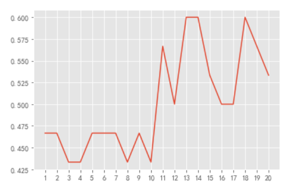
6.1 parameter learning curve
k in KNN is a super parameter. The so-called "super parameter" is a parameter that needs human input and cannot be calculated directly by the algorithm.
The parameter learning curve is a curve with different parameter values as abscissa and the model results under different parameter values as ordinate. We often choose the parameter value of the best performance point of the model as the value of this parameter.
#Prepare dataset
import pandas as pd
import numpy as np

data1 = pd.DataFrame(
    data=np.random.randint(0,100,size=(100,3)),
    columns=['A','B','C']
)
data2 = pd.DataFrame(
    data=np.random.randint(0,2,size=(100,1)),
    columns=['sex']
)
data1['y']=data2
print(data1)

#2.1 Guide Package
from sklearn.neighbors import KNeighborsClassifier
from sklearn.model_selection import train_test_split
#2.2 divide the data set, 30% as the test set and 70% as the training set
X = data1.iloc[:,0:-1] #Characteristic data
y = data1.iloc[:,-1]   #Label data
#The function returns 4 values: training feature, test feature, training tag and test tag
Xtrain,Xtest,ytrain,ytest = train_test_split(X,y,test_size=0.3,random_state=420) #test_size represents the size of the test set, random_state is similar to random Seed random seed

#2.3 modeling
KNN = KNeighborsClassifier(n_neighbors=22)
#2.4 classifier / training model
KNN = KNN.fit(Xtrain,ytrain)
#2.5 test accuracy using test sets
score = KNN.score(Xtest,ytest)
print(score) #Accuracy = 0.433335
print('========================================')

############################################################################################################
#Draw learning curve
#Value of x-axis K
#y-axis accuracy

x = []
y = []
for k in range(1,21): #
    x.append(k)
    clf = KNeighborsClassifier(n_neighbors=k)
    clf = clf.fit(Xtrain,ytrain)
    sc = clf.score(Xtest,ytest)
    y.append(sc)

print(x)
print(y)

#Drawing
import matplotlib.pyplot as plt
plt.plot(x,y)
plt.xticks(range(1,21))
plt.show()
6.2 cross validation
The model needs to consider two issues:
1. Accuracy, depending on K value
2. Stability, depending on the high scores in different data sets (if the scores in different data sets differ greatly, it indicates instability)
Unstable performance: when changing the random seed, the highest score K value of the model will change
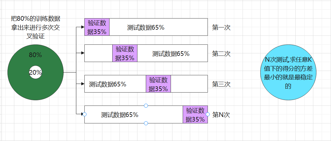
K-fold cross validation
The most commonly used cross validation is k-fold cross validation. We know that the division of training set and test set will interfere with the results of the model, so we use cross test
The mean value obtained from the results of n times is a better measure of the effect of the model.
schematic diagram:
6.3 parameter learning curve with cross validation
Objective: to find the K value with high score and small variance (both accuracy and stability)
K-fold cross validation code implementation:
#Prepare dataset
import pandas as pd
import numpy as np

data1 = pd.DataFrame(
    data=np.random.randint(0,100,size=(100,3)),
    columns=['A','B','C']
)
data2 = pd.DataFrame(
    data=np.random.randint(0,2,size=(100,1)),
    columns=['sex']
)
data1['y']=data2
print(data1)

#2.1 Guide Package
from sklearn.neighbors import KNeighborsClassifier
from sklearn.model_selection import train_test_split
from sklearn.model_selection import cross_val_score
#2.2 divide the data set, 30% as the test set and 70% as the training set
X = data1.iloc[:,0:-1] #Characteristic data
y = data1.iloc[:,-1]   #Label data
#The function returns 4 values: training feature, test feature, training tag and test tag
Xtrain,Xtest,ytrain,ytest = train_test_split(X,y,test_size=0.3,random_state=420) #test_size represents the size of the test set, random_state is similar to random Seed random seed

#3. Modeling
score=[] #Used to store the average score of each K-fold
var=[] #Used to store the fractional variance of each K-fold
K = [] #Value of stored K value
for i in range(1,21):
    KNN = KNeighborsClassifier(n_neighbors=i)
    #Cross validation
    result = cross_val_score(KNN,Xtrain,ytrain,cv=8) # cv=8 represents the number of K-turns
    K.append(i)
    score.append(result.mean())
    var.append(result.var())

print('K value',K)
print('mean value',score)
print('variance',var)

#4. Drawing
import matplotlib.pyplot as plt
#Convert the list into an array to perform mathematical operations
score = np.array(score)
var= np.array(var)
plt.plot(K,score,color='k')
plt.plot(K,score+var,color='r',linestyle='--')
plt.plot(K,score-var,color='b',linestyle='--')
plt.xticks(range(1,21))
Model interpretation:
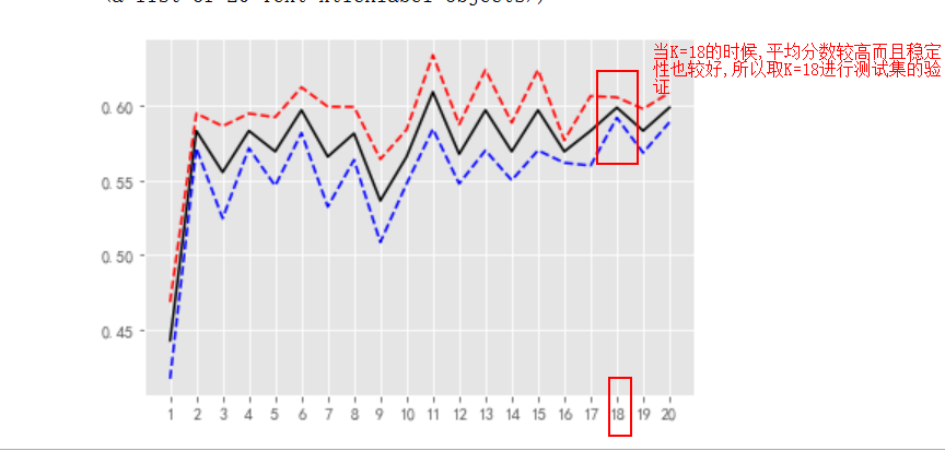
Test set validation:
#Test set validation

KNN_18 = KNeighborsClassifier(n_neighbors=18)
#Training model
fit = KNN_18.fit(Xtrain,ytrain)
#Test set verification score
sc = fit.score(Xtest,ytest)
sc #0.43333333333333335
be careful:
1. Do not set the K value too large, otherwise under fitting will occur, and too small will be over fitting
2.cv, that is, the number of folds of K cannot be too large or too small. In the function, the default = 5 folds, and the empirical value = 5 / 6 folds
Excessive discount:
Computational efficiency slows down.
The variance of prediction rate becomes larger, so it is difficult to ensure the expected prediction rate in the new data set.
Other cross validation:
All cross validation is based on the segmentation of training set and test set, but focuses on different directions
"k-fold" is to take the training set and test set in order
ShuffleSplit focuses on Distributing the test set in all directions of the data
Structured kfold believes that training data and test data must occupy the same proportion in each label classification
7: Normalization
When the data (x) is centered according to the minimum value and then scaled according to the range (maximum - Minimum), the data moves by the minimum value units and will be received
Converge to [0,1], and this process is called data Normalization (also known as min max scaling).
Objective: to eliminate the influence of dimension
Especially in the calculation of distance (such as PCA, such as KNN, such as kmeans, etc.), it is either normalized or standardized
Formula:
The first
one
species
square
type
:
(
X
i
−
X
m
i
n
)
/
(
X
m
a
x
−
X
m
i
n
)
The first
two
species
square
type
:
y
=
l
o
g
10
(
x
)
The first method: (X_i-X_min) / (X_max - X_min) \ \ the second method: y = log10(x)
The first method: (Xi − Xm in)/(Xm ax − Xm in) the second method: y=log10(x)
When to do normalization???
- First divided into training set and test set, and then normalized!
Normalization code implementation:
#Prepare dataset
import pandas as pd
import numpy as np

data1 = pd.DataFrame(
    data=np.random.randint(0,100,size=(100,3)),
    columns=['A','B','C']
)
data2 = pd.DataFrame(
    data=np.random.randint(0,2,size=(100,1)),
    columns=['sex']
)
data1['y']=data2
print(data1)

#2.1 Guide Package
from sklearn.neighbors import KNeighborsClassifier
from sklearn.model_selection import train_test_split
from sklearn.model_selection import cross_val_score
#2.2 divide the data set, 30% as the test set and 70% as the training set
X = data1.iloc[:,0:-1] #Characteristic data
y = data1.iloc[:,-1]   #Label data
#The function returns 4 values: training feature, test feature, training tag and test tag
Xtrain,Xtest,ytrain,ytest = train_test_split(X,y,test_size=0.3,random_state=420) #test_size represents the size of the test set, random_state is similar to random Seed random seed

#3. Normalization (first divide the data set, then normalize, and finally model)
from sklearn.preprocessing import MinMaxScaler as mms
Xtrain = mms().fit(Xtrain).transform(Xtrain)#Training set normalization
Xtest = mms().fit(Xtest).transform(Xtest)#Test set normalization
print(Xtrain_mms)


#3. Modeling
score=[] #Used to store the average score of each K-fold
var=[] #Used to store the fractional variance of each K-fold
K = [] #Value of stored K value
for i in range(1,21):
    KNN = KNeighborsClassifier(n_neighbors=i)
    #Cross validation
    result = cross_val_score(KNN,Xtrain,ytrain,cv=8) # cv=8 represents the number of K-turns
    K.append(i)
    score.append(result.mean())
    var.append(result.var())

print('K value',K)
print('mean value',score)
print('variance',var)

#4. Drawing
import matplotlib.pyplot as plt
#Convert the list into an array to perform mathematical operations
score = np.array(score)
var= np.array(var)
plt.plot(K,score,color='k')
plt.plot(K,score+var,color='r',linestyle='--')
plt.plot(K,score-var,color='b',linestyle='--')
plt.xticks(range(1,21))
8: Punishment of distance
Usage scenario: when the sample distribution is uneven
That is, set the weight according to the distance
It should be noted here that the optimization method of the model is only in theory, and the optimization will improve the discrimination effectiveness of the model, but in practical application
Whether the process can play a role ultimately depends essentially on the fit between the optimization method and the actual data. If the data itself exists
If there are a large number of outliers, using distance as the punishment factor will have a better effect, otherwise.
Code implementation:
- Kneigborsclassifier (n_neighbors = I, weights = 'distance') # weights = 'distance' stands for distance penalty
#Prepare dataset
import pandas as pd
import numpy as np

data1 = pd.DataFrame(
    data=np.random.randint(0,100,size=(100,3)),
    columns=['A','B','C']
)
data2 = pd.DataFrame(
    data=np.random.randint(0,2,size=(100,1)),
    columns=['sex']
)
data1['y']=data2
print(data1)

#2.1 Guide Package
from sklearn.neighbors import KNeighborsClassifier
from sklearn.model_selection import train_test_split
from sklearn.model_selection import cross_val_score
#2.2 divide the data set, 30% as the test set and 70% as the training set
X = data1.iloc[:,0:-1] #Characteristic data
y = data1.iloc[:,-1]   #Label data
#The function returns 4 values: training feature, test feature, training tag and test tag
Xtrain,Xtest,ytrain,ytest = train_test_split(X,y,test_size=0.3,random_state=420) #test_size represents the size of the test set, random_state is similar to random Seed random seed

#3. Normalization
from sklearn.preprocessing import MinMaxScaler as mms
Xtrain = mms().fit(Xtrain).transform(Xtrain)#Training set normalization
Xtest = mms().fit(Xtest).transform(Xtest)#Test set normalization
print(Xtrain_mms)


#3. Modeling + distance penalty
score=[] #Used to store the average score of each K-fold
var=[] #Used to store the fractional variance of each K-fold
K = [] #Value of stored K value
for i in range(1,21):
    KNN = KNeighborsClassifier(n_neighbors=i,weights='distance') # weights='distance 'stands for distance penalty
    #Cross validation
    result = cross_val_score(KNN,Xtrain,ytrain,cv=8) # cv=8 represents the number of K-turns
    K.append(i)
    score.append(result.mean())
    var.append(result.var())

print('K value',K)
print('mean value',score)
print('variance',var)

#4. Drawing
import matplotlib.pyplot as plt
#Convert the list into an array to perform mathematical operations
score = np.array(score)
var= np.array(var)
plt.plot(K,score,color='k')
plt.plot(K,score+var,color='r',linestyle='--')
plt.plot(K,score-var,color='b',linestyle='--')
plt.xticks(range(1,21))
N = kneigborsclassifier (n_neighbors = I, weights = 'distance') # weights = 'distance' stands for distance penalty
#Cross validation
result = cross_val_score(KNN,Xtrain,ytrain,cv=8) # cv=8 represents the number of K-turns
K.append(i)
score.append(result.mean())
var.append(result.var())
print('k value ', K)
print('mean ', score)
print('variance ', var)
#4. Drawing
import matplotlib.pyplot as plt
#Convert the list into an array to perform mathematical operations
score = np.array(score)
var= np.array(var)
plt.plot(K,score,color='k')
plt.plot(K,score+var,color='r',linestyle='–')
plt.plot(K,score-var,color='b',linestyle='–')
plt.xticks(range(1,21))