1, Linear SVM

1.1 maximum spacing and classification

Find a hyperplane in the sample space to separate different types of samples. At the same time, this line should be as far away from the sample points as possible. Then, this line is in the middle of the two sample points at the edge, and the sample points at these edges are called support vectors.

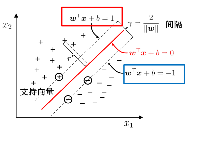
To find the maximum interval is to find the distance between two points. The distance between the positive and negative sample support vectors is equal to twice the distance from the positive sample to the classification line.

Where, molecule = 1
Get distance:

Finally, the problem becomes a solution
If the absolute value of the points of the above known support vectors is 1, the points after them should be > = 1
The following formula is easy to prove: if the classification is correct, then the value of yi is in the same direction as the value to be entered.

Convert to minimum

1.2 dual problem

The Lagrange multiplier method is used to find the minimum value under constraints


When SVM solves the w minimum value, the following steps are obtained:

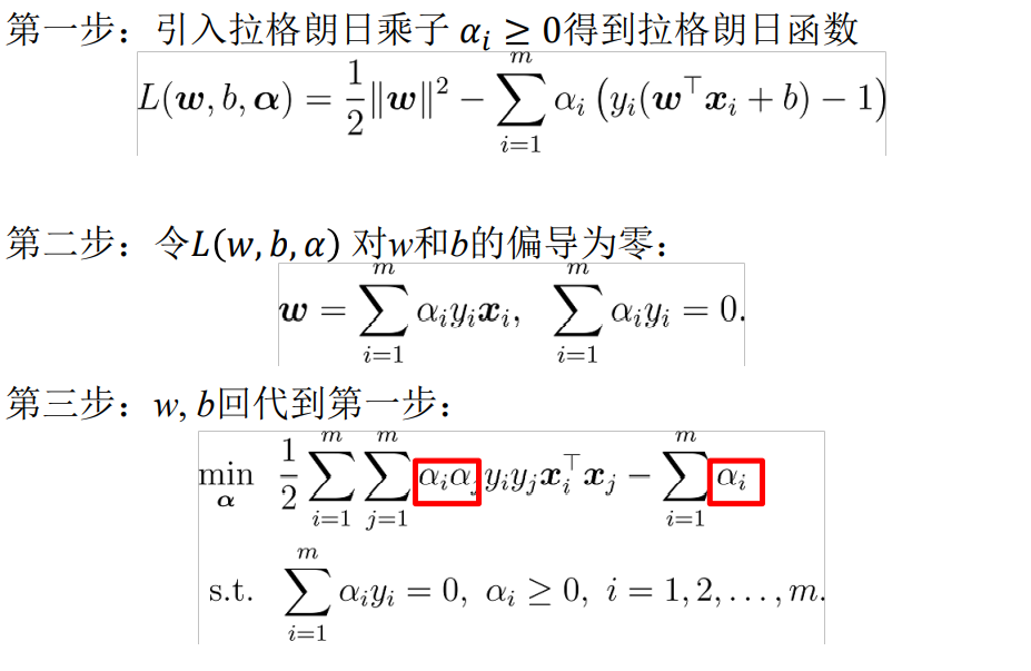
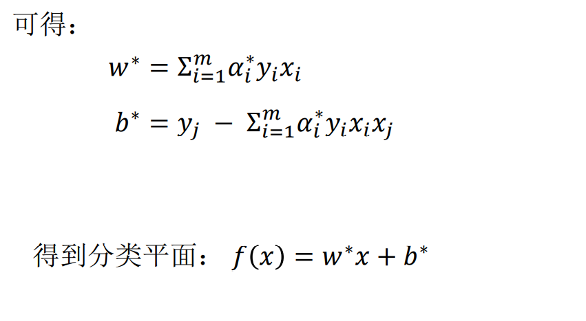
In the end, there are only unknowns left α i

1.3 SMO algorithm flow

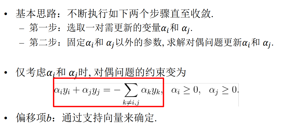
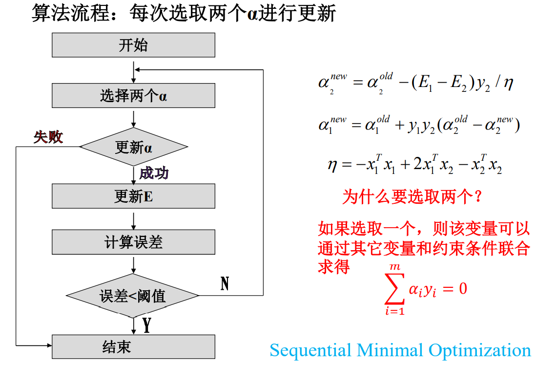
Finally solve α

2, Nonlinear SVM

2.1 kernel functions and kernel techniques

When the linearity is inseparable, a kernel function is selected to map it to a high-dimensional space to make it linearly separable

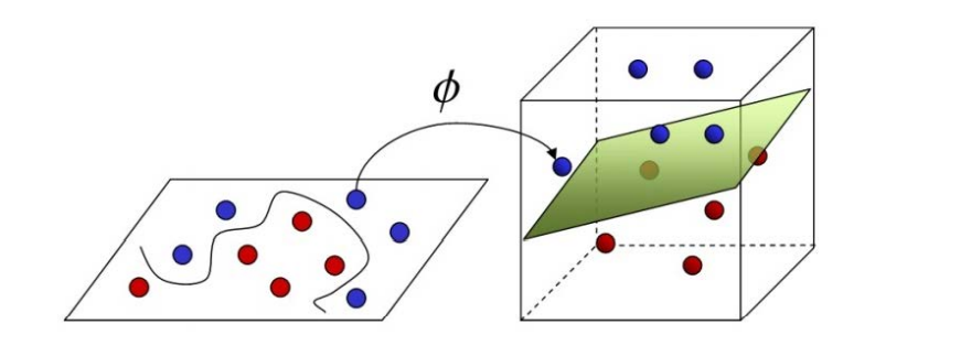
Among them, ϕ Yes, let the vector after sample x mapping be ϕ (x) , the partition hyperplane is f(x)=wT ϕ (x)+b

In this way, solving the problem is divided into two steps:
Firstly, a nonlinear mapping is used to transform the data into a feature space F;
Then, linear learner is used in feature space.
Common kernel functions are as follows:

If there is a method, the inner product can be calculated directly in the feature space< ϕ (x_i), ϕ (x) >, just as in the function of the original input point, it is possible to integrate the two steps to establish a sub linear learner. The direct calculation method is called kernel function method.
The method of replacing inner product with kernel function is called kernel trick.

2.3 soft interval and regularization

In practical application, it is difficult to select an appropriate kernel function to make the samples linearly separable in the feature space
Points; In addition, it is difficult to determine whether the linearly separable results are caused by over fitting. Therefore, the concept of "soft interval" is introduced to allow SVM to not meet the constraints on some samples.


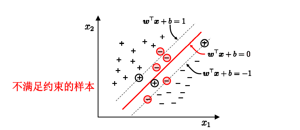
While solving the maximum interval, the samples that do not meet the constraints should be as few as possible, and finally turn to the solution

Where C > 0 is the penalty parameter

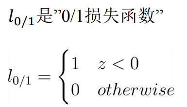
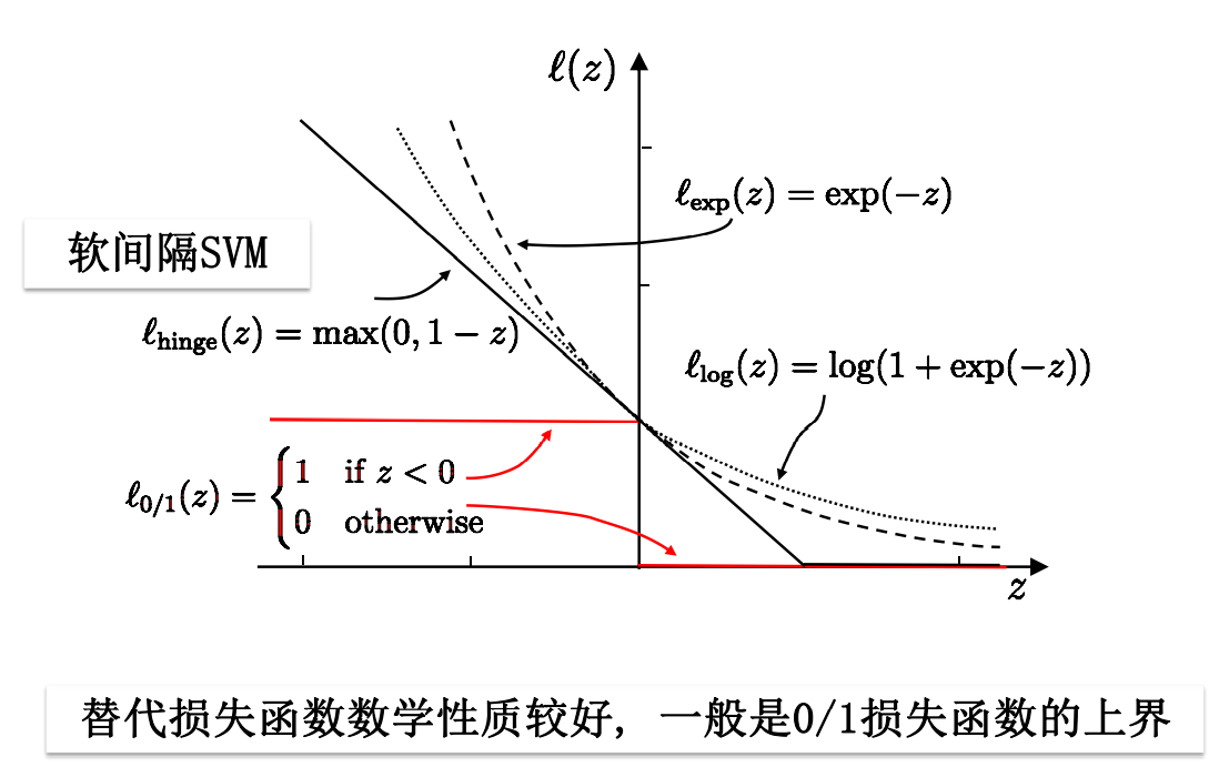
However, the loss function has some defects: nonconvex, discontinuous and difficult to optimize, so it is used to replace the loss function.

2.4 support vector regression

Support vector regression allows 2 between model output and actual output ε Deviation of

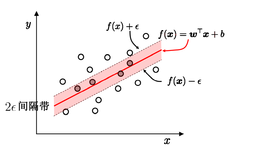
Among them, ε Is a relaxation variable, which reflects the tolerance of outliers

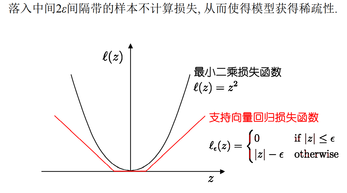
So the solution becomes:

3, Code practice

3.1 data preparation

It is the same as the dataset selected by logistic last time
The data set comes from the beast under sklearn_ Cancer, the breast cancer dataset.
There are 569 data in total, and there are two results: 0 is malignant and 1 is benign
There are 30 features.
This time, only the first 100 were selected, 85 were used as data sets, and 15 were tested.

3.2 algorithm implementation

data structure

class optStruct:
    """
	Data structure to maintain all values that need to be operated
	Parameters: 
		dataMatIn - Data matrix
		classLabels - Data label
		C - Relaxation variable
		toler - Fault tolerance rate
		kTup - Tuple containing kernel information,The first parameter stores the kernel function category, and the second parameter stores the parameters required by the necessary kernel function
	"""

    def __init__(self, dataMatIn, classLabels, C, toler, kTup):
        self.X = dataMatIn  # Data matrix
        self.labelMat = classLabels  # Data label
        self.C = C  # Relaxation variable - > tolerance to outliers
        self.tol = toler  # Fault tolerance rate
        self.m = np.shape(dataMatIn)[0]  # Data matrix rows
        self.alphas = np.mat(np.zeros((self.m, 1)))  # Initialize the alpha parameter to 0 according to the number of rows of the matrix
        self.b = 0  # Initialization b parameter is 0
        self.eCache = np.mat(np.zeros((self.m, 2)))  # Initialize the error buffer according to the number of rows of the matrix. The first column is the valid flag bit, and the second column is the value of the actual error E.
        self.K = np.mat(np.zeros((self.m, self.m)))  # Initialize kernel K
        for i in range(self.m):  # Calculate the kernel K of all data
            self.K[:, i] = kernelTrans(self.X, self.X[i, :], kTup)

Calculate the kernel function, and convert the data into higher dimensional space through the kernel function

def kernelTrans(X, A, kTup):
    
    m, n = np.shape(X)
    K = np.mat(np.zeros((m, 1)))
    if kTup[0] == 'lin':
        K = X * A.T  # Linear kernel function, only inner product.
    elif kTup[0] == 'rbf':  # Gaussian kernel function, calculated according to the Gaussian kernel function formula
        for j in range(m):
            deltaRow = X[j, :] - A
            K[j] = deltaRow * deltaRow.T
        K = np.exp(K / (-1 * kTup[1] ** 2))  # Computing Gaussian kernel K
    else:
        raise NameError('Kernel unrecognized')
    return K  # Returns the calculated kernel K

smo algorithm

def smoP(dataMatIn, classLabels, C, toler, maxIter, kTup=('lin', 0)):
    
    oS = optStruct(np.mat(dataMatIn), np.mat(classLabels).transpose(), C, toler, kTup)  # Initialize data structure
    iter = 0  # Initialize current iterations
    entireSet = True
    alphaPairsChanged = 0
    while (iter < maxIter) and ((alphaPairsChanged > 0) or (entireSet)):  # If the alpha of the entire dataset is not updated or the maximum number of iterations is exceeded, exit the loop
        alphaPairsChanged = 0
        if entireSet:  # Traverse the entire dataset
            for i in range(oS.m):
                alphaPairsChanged += innerL(i, oS)  # Using optimized SMO algorithm
                print("Full sample traversal:The first%d Second iteration sample:%d, alpha Optimization times:%d" % (iter, i, alphaPairsChanged))
            iter += 1
        else:  # Traversal of non boundary values
            nonBoundIs = np.nonzero((oS.alphas.A > 0) * (oS.alphas.A < C))[0]  # Traverse alpha not at boundaries 0 and C
            for i in nonBoundIs:
                alphaPairsChanged += innerL(i, oS)
                print("Non boundary traversal:The first%d Second iteration sample:%d, alpha Optimization times:%d" % (iter, i, alphaPairsChanged))
            iter += 1
        if entireSet:  # After traversing once, it is changed to non boundary traversal
            entireSet = False
        elif (alphaPairsChanged == 0):  # If the alpha is not updated, the full sample traversal is calculated
            entireSet = True
        print("Number of iterations: %d" % iter)
    return oS.b, oS.alphas  # Returns b and alpha calculated by SMO algorithm

Optimized smo algorithm

def innerL(i, oS):
    
    # Step 1: calculate the error Ei
    Ei = calcEk(oS, i)
    # Optimize alpha and set a certain fault tolerance rate.
    if ((oS.labelMat[i] * Ei < -oS.tol) and (oS.alphas[i] < oS.C)) or (
            (oS.labelMat[i] * Ei > oS.tol) and (oS.alphas[i] > 0)):
        # Select alpha using inner loop heuristic method 2_ j. And calculate Ej
        j, Ej = selectJ(i, oS, Ei)
        # Save the aplpha value before update and use deep copy
        alphaIold = oS.alphas[i].copy()
        alphaJold = oS.alphas[j].copy()
        # Step 2: calculate the upper and lower bounds L and H
        if (oS.labelMat[i] != oS.labelMat[j]):
            L = max(0, oS.alphas[j] - oS.alphas[i])
            H = min(oS.C, oS.C + oS.alphas[j] - oS.alphas[i])
        else:
            L = max(0, oS.alphas[j] + oS.alphas[i] - oS.C)
            H = min(oS.C, oS.alphas[j] + oS.alphas[i])
        if L == H:
            print("L==H")
            return 0
        # Step 3: calculate eta
        eta = 2.0 * oS.K[i, j] - oS.K[i, i] - oS.K[j, j]
        if eta >= 0:
            print("eta>=0")
            return 0
        # Step 4: update alpha_j
        oS.alphas[j] -= oS.labelMat[j] * (Ei - Ej) / eta
        # Step 5: trim alpha_j
        oS.alphas[j] = clipAlpha(oS.alphas[j], H, L)
        # Update Ej to error cache
        updateEk(oS, j)
        if (abs(oS.alphas[j] - alphaJold) < 0.00001):
            print("alpha_j The change is too small")
            return 0
        # Step 6: update alpha_i
        oS.alphas[i] += oS.labelMat[j] * oS.labelMat[i] * (alphaJold - oS.alphas[j])
        # Update Ei to error cache
        updateEk(oS, i)
        # Step 7: update b_1 and B_ two
        b1 = oS.b - Ei - oS.labelMat[i] * (oS.alphas[i] - alphaIold) * oS.K[i, i] - oS.labelMat[j] * (
                oS.alphas[j] - alphaJold) * oS.K[i, j]
        b2 = oS.b - Ej - oS.labelMat[i] * (oS.alphas[i] - alphaIold) * oS.K[i, j] - oS.labelMat[j] * (
                oS.alphas[j] - alphaJold) * oS.K[j, j]
        # Step 8: according to b_1 and b_2 update b
        if (0 < oS.alphas[i]) and (oS.C > oS.alphas[i]):
            oS.b = b1
        elif (0 < oS.alphas[j]) and (oS.C > oS.alphas[j]):
            oS.b = b2
        else:
            oS.b = (b1 + b2) / 2.0
        return 1
    else:
        return 0

calculation error

def calcEk(oS, k):
   
    fXk = float(np.multiply(oS.alphas, oS.labelMat).T * oS.K[:, k] + oS.b)
    Ek = fXk - float(oS.labelMat[k])
    return Ek

Calculation of Ej by inner loop heuristic method

def selectJ(i, oS, Ei):
    
    maxK = -1
    maxDeltaE = 0
    Ej = 0  # initialization
    oS.eCache[i] = [1, Ei]  # Update error cache according to Ei
    validEcacheList = np.nonzero(oS.eCache[:, 0].A)[0]  # Returns the index value of data whose error is not 0
    if (len(validEcacheList)) > 1:  # There is an error that is not 0
        for k in validEcacheList:  # Traverse to find the maximum Ek
            if k == i: continue  # Not counting i is a waste of time
            Ek = calcEk(oS, k)  # Calculate Ek
            deltaE = abs(Ei - Ek)  # Calculate | EI EK|
            if (deltaE > maxDeltaE):  # maxDeltaE found
                maxK = k
                maxDeltaE = deltaE
                Ej = Ek
        return maxK, Ej  # Return maxK,Ej
    else:  # There is no error that is not 0
        j = selectJrand(i, oS.m)  # Randomly select alpha_ Index value of J
        Ej = calcEk(oS, j)  # Calculate Ej
    return j, Ej  # j,Ej

Trim alpha_j

def clipAlpha(aj, H, L):
    
    if aj > H:
        aj = H
    if L > aj:
        aj = L
    return aj

Update Ej to error cache

def updateEk(oS, k):
    """
	calculation Ek,And update the error buffer
	Parameters: 
		oS - data structure
		k - Label is k Index value of the data
	Returns:
		nothing
	"""
    Ek = calcEk(oS, k)  # Calculate Ek
    oS.eCache[k] = [1, Ek]  # Update error cache

3.3 operation results and analysis

The error rate is as follows:

The error rate of the test set is high, and there may be too many guessed attributes (30), which makes it difficult to classify
Even if the book data is used, with only two attributes, the error rate of the test set is twice that of the data set

Therefore, there are many possible changes in the code.

4, Summary

SVM is very difficult from principle to code implementation. It is still not well understood. We need to strengthen its learning in the future.