- Practice purpose
Be familiar with the application of iterative method in meteorology, and master the actual programming and calculation of stability index.
- Practice content
1. It is known that the 6h reanalysis data in 2020 include temperature, height, relative humidity and horizontal wind field. The pseudo equivalent potential temperature at 20 o'clock on each day (the second day of each team's responsible date) of each layer in a certain area (10 º N-60 º N,60 º E-140 º E) is calculated by iterative method, and the corresponding diagrams at 850 and 500hPa and the difference between the two layers are given.
2. According to the 6h reanalysis data in 2020, the element fields include temperature, height, relative humidity and horizontal wind field. Calculate the pseudo phase equivalent temperature and potential temperature of each floor at 20:00 on each day (the second day of each team's responsible date) (70 º E-100 º E), (100 º E-110 º E) and (110 º E-120 º E) on the (10 º N-60 º N,1000-300hPa) plane, and give the corresponding diagram.
- Analysis of practice results
3.1 calculation procedure
(1) Calculate 850 hPa pseudo equivalent potential temperature, 500 hPa pseudo equivalent potential temperature and the difference between the two layers
(2) Calculate the pseudo phase equivalent temperature and potential temperature on the regional average (70 º E-100 º E), (100 º E-110 º E), (110 º E-120 º E), (10 º N-60 º N) of Beijing at 20:00 at 1000-300hPa
3.2 drawing program and description document of calculation
(1) Program code - calculate the pseudo phase equivalent temperature and potential temperature on the regional average (70 º E-100 º E), (100 º E-110 º E), (110 º E-120 º E), (10 º N-60 º N) of Beijing at 1000-300hPa at 12:00 on June 9 (the second day)
%read.nc Data data

%route

indir = 'E:\Day diagnosis\';

ncdisp([indir,'air.2020.nc']);

ncdisp([indir,'hgt.2020.nc']);

ncdisp([indir,'rhum.2020.nc']);

ncdisp([indir,'uwnd.2020.nc']);

ncdisp([indir,'vwnd.2020.nc']);

%variable

T=ncread(['E:\Day diagnosis\','air.2020.nc'],'air');%temperature T

H=ncread(['E:\Day diagnosis\','hgt.2020.nc'],'hgt');%height H

RH=ncread(['E:\Day diagnosis\','rhum.2020.nc'],'rhum');%relative humidity RH

u=ncread(['E:\Day diagnosis\','uwnd.2020.nc'],'uwnd');%Horizontal wind field u

v=ncread(['E:\Day diagnosis\','vwnd.2020.nc'],'vwnd');%Horizontal wind field v

%(4 dimension)Index variable-lon,lat,level,time

lon=ncread(['E:\Day diagnosis\','air.2020.nc'],'lon');

lat=ncread(['E:\Day diagnosis\','air.2020.nc'],'lat');

level=ncread(['E:\Day diagnosis\','air.2020.nc'],'level');

time=ncread(['E:\Day diagnosis\','air.2020.nc'],'time');

%10?N-60?N,100?E-140?E-925hPa In terms of air pressure - June 9 - 20:00 in Beijing - dew point temperature, condensation height, condensation temperature and time

timez=(datenum(2020,6,9,12,0,0)-datenum('1800-01-01 00:00:0.0'))*24; %Convert world 12 o'clock into data time

%Convert index subscript

time_z=find(time==timez);

level_z=find(level==850);

minlon=find(lon==100);

maxlon=find(lon==140);

minlat=find(lat==10);

maxlat=find(lat==60);

%Take out the required data(lon,lat,level,time)

TT=T(minlon:maxlon,maxlat:minlat,level_z,time_z);

HH=H(minlon:maxlon,maxlat:minlat,level_z,time_z);

RHRH=RH(minlon:maxlon,maxlat:minlat,level_z,time_z);

uu=u(minlon:maxlon,maxlat:minlat,level_z,time_z);

vv=v(minlon:maxlon,maxlat:minlat,level_z,time_z);


%Calculate dew point - previously programmed with the Celsius formula

RH=RHRH;tz=TT-273.15;e0=6.1078;a=17.269;b=35.86;

es=e0.*exp((a.*tz)./(273.16+tz-b));

ez=RH./100.*es;

for i=1:maxlon-minlon+1

    for j=1:minlat-maxlat+1

        while ez(i,j)-es(i,j)<0

              tz(i,j)=tz(i,j)-0.01;

              es(i,j)=e0.*exp((a.*tz(i,j))./(273.15+tz(i,j)-b));

        end

        td(i,j)=tz(i,j);

    end

end


%Calculation of pseudo equivalent potential temperature

RH=RHRH;Tz=TT;Td=td+273.15;P0=1000.0;Pz=925;Z=HH;e0=6.1078;a=17.269;b=35.86;Cp=1004;g=9.8;L=2.5*10^6; %2.5×10^6J/kg

ez=e0.*exp((a.*(Td-273.15))./(Td-b));

seita_z=Tz.*(P0./Pz).^0.286;

qz=0.622.*ez./(Pz-0.378.*ez);

for i=1:maxlon-minlon+1

    for j=1:minlat-maxlat+1

        Pl=300;

        Tl(i,j)=seita_z(i,j).*(Pl./P0).^0.286;

        el(i,j)=e0.*exp((a*(Tl(i,j)-273.15))/(Tl(i,j)-b));

        ql(i,j)=0.622.*el(i,j)/(Pl-0.378.*el(i,j));

        while ql(i,j)-qz(i,j)<0

        Pl=Pl+1;

        Tl(i,j)=seita_z(i,j).*(Pl./P0).^0.286;

        el(i,j)=e0.*exp((a*(Tl(i,j)-273.15))/(Tl(i,j)-b));

        ql(i,j)=0.622.*el(i,j)/(Pl-0.378.*el(i,j));

        end

        seita_se(i,j)=seita_z(i,j).*exp(L*qz(i,j)/(Cp.*Tl(i,j)));

    end

end

 %Draw a picture

m_proj('lambert','lon',[100 140],'lat',[10 60]); hold on

m_grid('linestyle','-','tickdir','out','linewidth',3); hold on

m_contourf(100:2.5:140,60:-2.5:10,seita_se',15,'linestyle','none'); hold on

colormap(m_colmap('jet',10));%Fill color matching

colorbar('Location','eastoutside');%Color bar

m_coast('color',[0 0 0]);%coastline-Black tricolor

hold on


seita_se=seita_se';

seita_se_=seita_se(21:-1:1,:)-273.15;

[C,h] = contourf(seita_se_,8);

clabel(C,h)
3.3 drawing graphics, statistical tables and related analysis
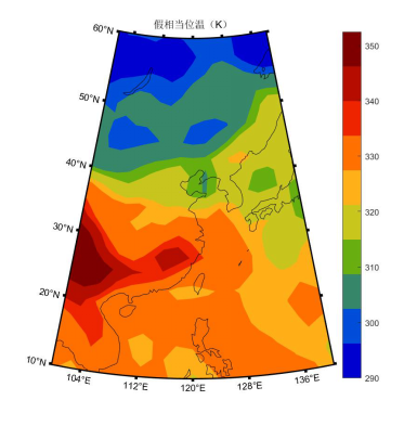
(1) The operation results of the first question are shown in the figure:
(2) The drawing result of the second question is shown in the figure:
- Second question: Result Analysis:
It can be seen from the last practice that the north side is low temperature, there is an area with high air saturation, and the south side is high temperature and high humidity. The warm and humid water vapor brought by the southeast air flow from the Pacific Ocean. There is a convergence area in 20N-30N and 112E-120E, with high temperature and humidity.
The range of pseudo equivalent potential temperature in the study area is 290-350K, there is a warm center in 20N-30N in the west, and there is a high value area in 20N-30N and 112E-120E. There is a low value area in the north, and the overall potential temperature distribution is difficult to warm and cold in the north.
3.4 existing problems or problems encountered or experience or summary
Because on the basis of reading the data for the first time, only a calculation formula is changed, so the part of calculation and programming can be changed. Problems encountered: the mapping map is difficult to overlay. Through online search for data and continuous attempts, the superposition of simple coastlines is more intuitive than the previous only longitude and latitude.