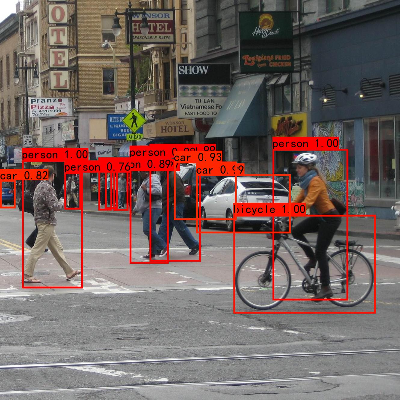
I believe that students who study algorithms will learn yoov1 algorithm when they are just getting started with target detection. After all, it is the beginning of YOLO algorithm. Of course, in order to take notes, they will do it directly on this blog for your reference and study. Next, I will share the knowledge required for the implementation of yolov1 algorithm:
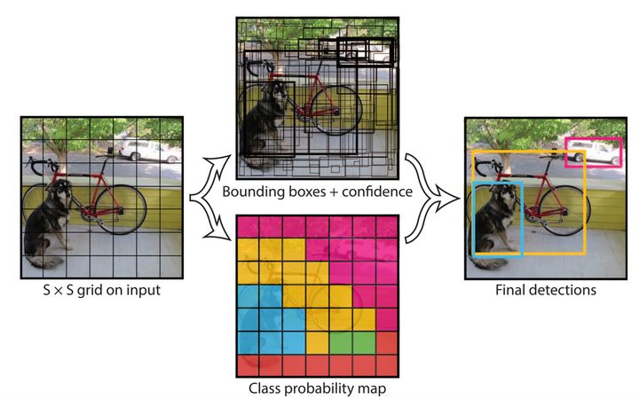
First of all, we have a general understanding of YOLOv1, that is, as shown in the figure below, by inputting a picture or a sequence of images (video) into the model (after training), we can directly complete the classification and positioning functions, such as the dog category and car category in the picture below, as well as their positions in the picture. The middle part is directly used as the model first. Don't think about it, Let's look at the following first. The relevant content of this article comes from YOLO - getting started from scratch - target detection - Zhihu , if necessary, you can also see the target detection algorithm described by the boss.
1, Data set
Data set is a key part of a code. If there is no data set and everything is empty, I directly recommend VOC2007/2012 and COCO data sets for target detection data sets. The following is my own download, so I also recommend it to you. Save you looking for it.
Link: https://pan.baidu.com/s/1niIAmSmoHa84aNywk-MZQw
Extraction code: 2222
Two, model architecture
First, let's take a look at the overall model of YOLOv1 algorithm, as shown in the following figure:
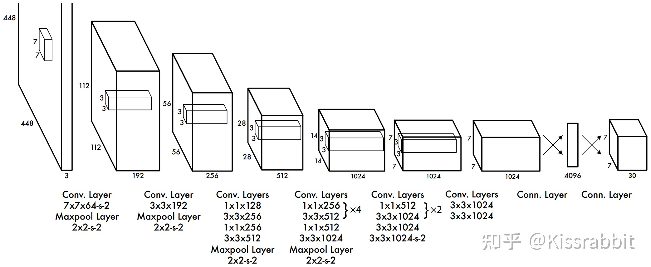
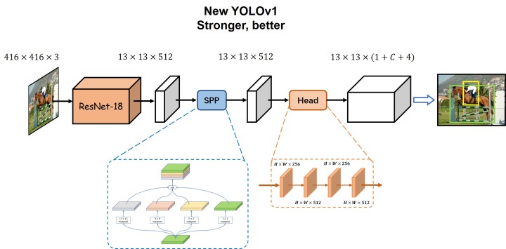
From the model, we can roughly see that a picture with the specification of [w,h,3] is scaled to the size of [448, 448, 3], and after convolution network, we get [7, 7, 30], where 7 represents the size of the feature map, and 30 can be divided into 1 + 4 + 20, where 1 represents the probability of whether there is an object, 4 represents the offset (tx,ty) and width height of the center point coordinate (note that this is either the offset or the normal value) (tw,th). Here is a code of this model:
import torch
import torch.nn as nn
import torch.utils.model_zoo as model_zoo
import torch.nn.functional as F
import numpy as np
__all__ = ['ResNet', 'resnet18', 'resnet34', 'resnet50', 'resnet101',
           'resnet152']

model_urls = {
    'resnet18': 'https://download.pytorch.org/models/resnet18-5c106cde.pth',
    'resnet34': 'https://download.pytorch.org/models/resnet34-333f7ec4.pth',
    'resnet50': 'https://download.pytorch.org/models/resnet50-19c8e357.pth',
    'resnet101': 'https://download.pytorch.org/models/resnet101-5d3b4d8f.pth',
    'resnet152': 'https://download.pytorch.org/models/resnet152-b121ed2d.pth',
}


def conv3x3(in_planes, out_planes, stride=1):
    """3x3 convolution with padding"""
    return nn.Conv2d(in_planes, out_planes, kernel_size=3, stride=stride,
                     padding=1, bias=False)


def conv1x1(in_planes, out_planes, stride=1):
    """1x1 convolution"""
    return nn.Conv2d(in_planes, out_planes, kernel_size=1, stride=stride, bias=False)


class BasicBlock(nn.Module):
    expansion = 1

    def __init__(self, inplanes, planes, stride=1, downsample=None):
        super(BasicBlock, self).__init__()
        self.conv1 = conv3x3(inplanes, planes, stride)
        self.bn1 = nn.BatchNorm2d(planes)
        self.relu = nn.ReLU(inplace=True)
        self.conv2 = conv3x3(planes, planes)
        self.bn2 = nn.BatchNorm2d(planes)
        self.downsample = downsample
        self.stride = stride

    def forward(self, x):
        identity = x

        out = self.conv1(x)
        out = self.bn1(out)
        out = self.relu(out)

        out = self.conv2(out)
        out = self.bn2(out)

        if self.downsample is not None:
            identity = self.downsample(x)

        out += identity
        out = self.relu(out)

        return out


class Bottleneck(nn.Module):
    expansion = 4

    def __init__(self, inplanes, planes, stride=1, downsample=None):
        super(Bottleneck, self).__init__()
        self.conv1 = conv1x1(inplanes, planes)
        self.bn1 = nn.BatchNorm2d(planes)
        self.conv2 = conv3x3(planes, planes, stride)
        self.bn2 = nn.BatchNorm2d(planes)
        self.conv3 = conv1x1(planes, planes * self.expansion)
        self.bn3 = nn.BatchNorm2d(planes * self.expansion)
        self.relu = nn.ReLU(inplace=True)
        self.downsample = downsample
        self.stride = stride

    def forward(self, x):
        identity = x

        out = self.conv1(x)
        out = self.bn1(out)
        out = self.relu(out)

        out = self.conv2(out)
        out = self.bn2(out)
        out = self.relu(out)

        out = self.conv3(out)
        out = self.bn3(out)

        if self.downsample is not None:
            identity = self.downsample(x)

        out += identity
        out = self.relu(out)

        return out


class ResNet(nn.Module):

    def __init__(self, block, layers, zero_init_residual=False):
        super(ResNet, self).__init__()
        self.inplanes = 64
        self.conv1 = nn.Conv2d(3, 64, kernel_size=7, stride=2, padding=3,
                               bias=False)
        self.bn1 = nn.BatchNorm2d(64)
        self.relu = nn.ReLU(inplace=True)
        self.maxpool = nn.MaxPool2d(kernel_size=3, stride=2, padding=1)
        self.layer1 = self._make_layer(block, 64, layers[0])
        self.layer2 = self._make_layer(block, 128, layers[1], stride=2)
        self.layer3 = self._make_layer(block, 256, layers[2], stride=2)
        self.layer4 = self._make_layer(block, 512, layers[3], stride=2)

        for m in self.modules():
            if isinstance(m, nn.Conv2d):
                nn.init.kaiming_normal_(m.weight, mode='fan_out', nonlinearity='relu')
            elif isinstance(m, nn.BatchNorm2d):
                nn.init.constant_(m.weight, 1)
                nn.init.constant_(m.bias, 0)

        # Zero-initialize the last BN in each residual branch,
        # so that the residual branch starts with zeros, and each residual block behaves like an identity.
        # This improves the model by 0.2~0.3% according to https://arxiv.org/abs/1706.02677
        if zero_init_residual:
            for m in self.modules():
                if isinstance(m, Bottleneck):
                    nn.init.constant_(m.bn3.weight, 0)
                elif isinstance(m, BasicBlock):
                    nn.init.constant_(m.bn2.weight, 0)

    def _make_layer(self, block, planes, blocks, stride=1):
        downsample = None
        if stride != 1 or self.inplanes != planes * block.expansion:
            downsample = nn.Sequential(
                conv1x1(self.inplanes, planes * block.expansion, stride),
                nn.BatchNorm2d(planes * block.expansion),
            )

        layers = []
        layers.append(block(self.inplanes, planes, stride, downsample))
        self.inplanes = planes * block.expansion
        for _ in range(1, blocks):
            layers.append(block(self.inplanes, planes))

        return nn.Sequential(*layers)

    def forward(self, x):
        C_1 = self.conv1(x)
        C_1 = self.bn1(C_1)
        C_1 = self.relu(C_1)
        C_1 = self.maxpool(C_1)

        C_2 = self.layer1(C_1)
        C_3 = self.layer2(C_2)
        C_4 = self.layer3(C_3)
        C_5 = self.layer4(C_4)

        return C_5


def resnet18(pretrained=False, **kwargs):
    """Constructs a ResNet-18 model.

    Args:
        pretrained (bool): If True, returns a model pre-trained on ImageNet
    """
    model = ResNet(BasicBlock, [2, 2, 2, 2], **kwargs)
    if pretrained:
        # strict = False as we don't need fc layer params.
        model.load_state_dict(model_zoo.load_url(model_urls['resnet18']), strict=False)
    return model


def resnet34(pretrained=False, **kwargs):
    """Constructs a ResNet-34 model.

    Args:
        pretrained (bool): If True, returns a model pre-trained on ImageNet
    """
    model = ResNet(BasicBlock, [3, 4, 6, 3], **kwargs)
    if pretrained:
        model.load_state_dict(model_zoo.load_url(model_urls['resnet34']), strict=False)
    return model


def resnet50(pretrained=False, **kwargs):
    """Constructs a ResNet-50 model.

    Args:
        pretrained (bool): If True, returns a model pre-trained on ImageNet
    """
    model = ResNet(Bottleneck, [3, 4, 6, 3], **kwargs)
    if pretrained:
        model.load_state_dict(model_zoo.load_url(model_urls['resnet50']), strict=False)
    return model


def resnet101(pretrained=False, **kwargs):
    """Constructs a ResNet-101 model.

    Args:
        pretrained (bool): If True, returns a model pre-trained on ImageNet
    """
    model = ResNet(Bottleneck, [3, 4, 23, 3], **kwargs)
    if pretrained:
        model.load_state_dict(model_zoo.load_url(model_urls['resnet101']), strict=False)
    return model


def resnet152(pretrained=False, **kwargs):
    """Constructs a ResNet-152 model.

    Args:
        pretrained (bool): If True, returns a model pre-trained on ImageNet
    """
    model = ResNet(Bottleneck, [3, 8, 36, 3], **kwargs)
    if pretrained:
        model.load_state_dict(model_zoo.load_url(model_urls['resnet152']))
    return model

#Build SPP module
class Conv(nn.Module):
    def __init__(self, c1, c2, k, s=1, p=0, d=1, g=1, act=True):
        super(Conv, self).__init__()
        self.convs = nn.Sequential(
            nn.Conv2d(c1, c2, k, stride=s, padding=p, dilation=d, groups=g),
            nn.BatchNorm2d(c2),
            nn.LeakyReLU(0.1, inplace=True) if act else nn.Identity()
        )

    def forward(self, x):
        return self.convs(x)


class SPP(nn.Module):
    """
        Spatial Pyramid Pooling
    """
    def __init__(self):
        super(SPP, self).__init__()

    def forward(self, x):
        x_1 = torch.nn.functional.max_pool2d(x, 5, stride=1, padding=2)
        x_2 = torch.nn.functional.max_pool2d(x, 9, stride=1, padding=4)
        x_3 = torch.nn.functional.max_pool2d(x, 13, stride=1, padding=6)
        x = torch.cat([x, x_1, x_2, x_3], dim=1)

        return x

#Build an overall network
class Yolov1(nn.Module):
    def __init__(self,num_class=20):
        super(Yolov1, self).__init__()
        self.num_class=num_class
        self.backbone=resnet18(pretrained=False)
        c5 = 512
        self.neck = nn.Sequential(
            SPP(),
            Conv(c5 * 4, c5, k=1),
        )
        # detection head
        self.convsets = nn.Sequential(
            Conv(c5, 256, k=1),
            Conv(256, 512, k=3, p=1),
            Conv(512, 256, k=1),
            Conv(256, 512, k=3, p=1)
        )
        # detection head
        self.convsets = nn.Sequential(
            Conv(c5, 256, k=1),
            Conv(256, 512, k=3, p=1),
            Conv(512, 256, k=1),
            Conv(256, 512, k=3, p=1)
        )
        # pred
        self.pred = nn.Conv2d(512, 1 + self.num_class + 4, 1)

    def forward(self,x):
        B,C,W,H=x.shape
        # backbone network
        c5 = self.backbone(x)

        # neck network
        p5 = self.neck(c5)

        # detection head network
        p5 = self.convsets(p5)

        # Prediction layer
        pred = self.pred(p5)

        pred=pred.view(B,pred.size(1),-1).permute(0, 2, 1)

        conf_pred=pred[...,0:1]
        cls_pred = pred[...,1:1+self.num_class]
        # bbox prediction: [B, H*W, 4]
        txtytwth_pred = pred[...,1 + self.num_class:]
        return pred,conf_pred,cls_pred,txtytwth_pred
Note: I believe you have read other people'S blogs and said that a picture is divided into SXS grids. I believe you are a little confused. Let me explain that it is actually the [7,7,30] we just got. We regard 7x7 as a piece of paper, and then there are 30 pieces of 7x7 paper. Then in this piece of 7x7 paper, we can regard it as 49 grids, Then each grid will contain the receptive field size of the original picture (448 / 7448 / 7). Therefore, there are 49 grids (448 / 7448 / 7) in the whole input picture. Now we can understand S as 7.
3, Value of positive and negative samples
For the pictures and labels given by the data set, that is, the objects to be detected in a picture will be labeled to you, that is, the relevant data of the real box will be given to you. Then what you need to do is to process the data, send it to the network and calculate the loss function. Then you need to process the label to make the center coordinate become the offset value, which is convenient for convergence.
def generate_dxdywh(gt_label, w, h, s):
    xmin, ymin, xmax, ymax = gt_label[:-1]
    # Calculate the center point of the bounding box
    c_x = (xmax + xmin) / 2 * w
    c_y = (ymax + ymin) / 2 * h
    box_w = (xmax - xmin) * w
    box_h = (ymax - ymin) * h

    if box_w < 1e-4 or box_h < 1e-4:#Just to verify whether the length and width are qualified
        # print('Not a valid data !!!')
        return False

    # Calculate the grid coordinates of the center point
    c_x_s = c_x / s
    c_y_s = c_y / s
    grid_x = int(c_x_s)
    grid_y = int(c_y_s)
    # Label for calculating center point offset and width and height
    tx = c_x_s - grid_x
    ty = c_y_s - grid_y
    tw = np.log(box_w)
    th = np.log(box_h)
    # Calculate the loss weight of the bounding box position parameter
    weight = 2.0 - (box_w / w) * (box_h / h)

    return grid_x, grid_y, tx, ty, tw, th, weight


def gt_creator(input_size, stride, label_lists=[]):
    # Necessary parameters
    batch_size = len(label_lists)
    w = input_size
    h = input_size
    ws = w // stride
    hs = h // stride
    s = stride
    gt_tensor = np.zeros([batch_size, hs, ws, 1+1+4+1])

    # Make training labels
    for batch_index in range(batch_size):
        for gt_label in label_lists[batch_index]:
            gt_class = int(gt_label[-1])
            result = generate_dxdywh(gt_label, w, h, s)
            if result:
                grid_x, grid_y, tx, ty, tw, th, weight = result

                if grid_x < gt_tensor.shape[2] and grid_y < gt_tensor.shape[1]:#If the coordinates of the upper left corner of the real box are consistent with the set grid, the label is qualified.
                    gt_tensor[batch_index, grid_y, grid_x, 0] = 1.0
                    gt_tensor[batch_index, grid_y, grid_x, 1] = gt_class
                    gt_tensor[batch_index, grid_y, grid_x, 2:6] = np.array([tx, ty, tw, th])
                    gt_tensor[batch_index, grid_y, grid_x, 6] = weight


    gt_tensor = gt_tensor.reshape(batch_size, -1, 1+1+4+1)

    return torch.from_numpy(gt_tensor).float()
Note: in other blogs, you will see that the central point of the object falls on that grid, that is, there is that grid to return to the target box. In fact, its meaning is easy to interpret, that is, now that we have the information of the real box, we can know the grid position of the central point of the real box. As for why the word grid appears again, That's what I explained above. Grid can be generated by code. Here is the code. Then, after the grid position is obtained, the predicted value can also be known through the network. We change the predicted value into the size relative to the input picture through the relevant formula, but the predicted value will certainly exist in each grid, Then we just need to take the grid where the center coordinate of the real value is located as the predicted value of the same position as the grid for loss calculation, which is the meaning of that sentence. I believe everyone knows. Here's the code.
#Build grid
def create_grid(input_size,stride):#224x224
    input_w,input_h=input_size
    grid_w,grid_h=input_w//stride,input_ H / / stripe # assuming stripe = 32, grid_w,grid_h=7,7
    #Create grid sequence number
    grid_x,grid_y=torch.meshgrid(torch.arange(grid_w),torch.arange(grid_h))
    grid_xy=torch.stack([grid_x,grid_y],dim=-1).float()
    grid_xy = grid_xy.view(1, grid_w * grid_h, 2)
    return grid_xy
IV. loss calculation
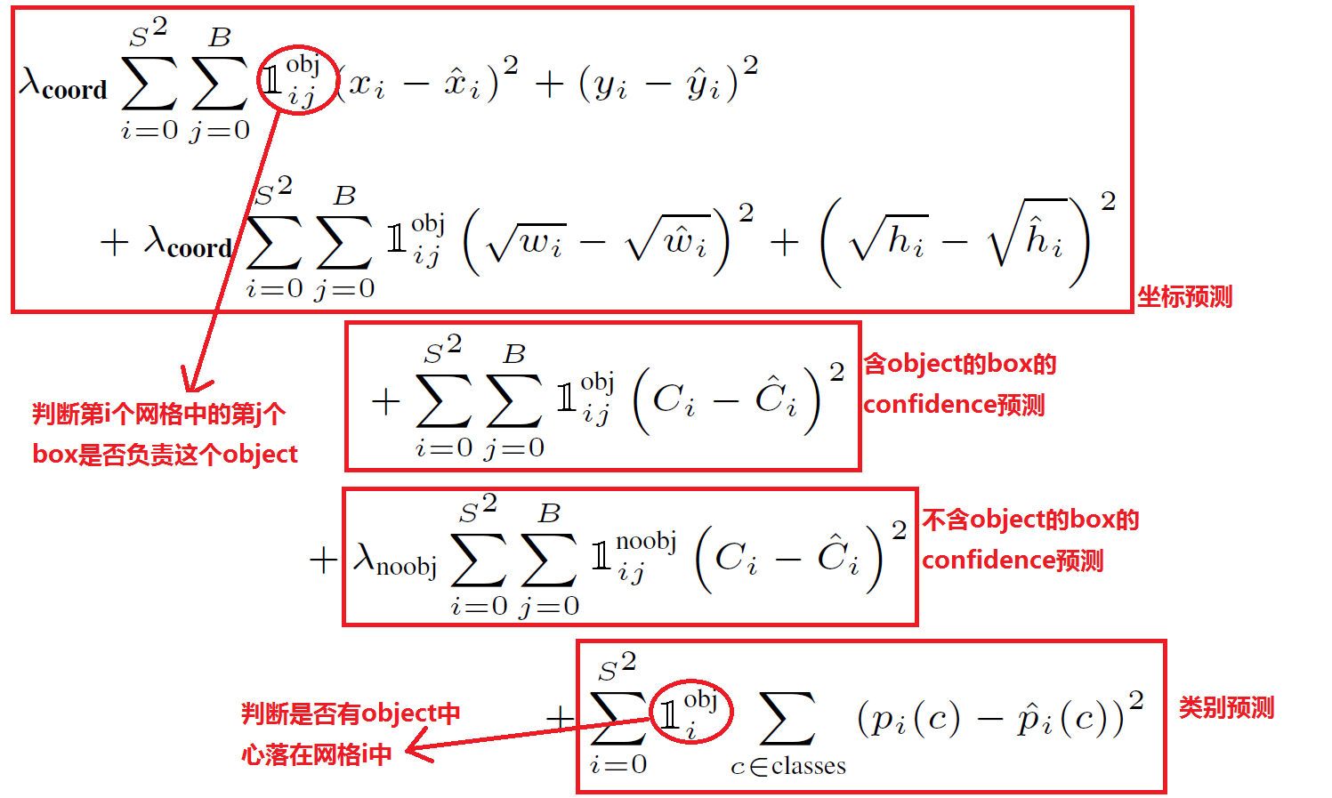
Loss calculation is the top priority of an algorithm. If there is no loss calculation, the algorithm will come to an end. We can see from the loss calculation diagram that the former coefficient is remembered to balance the effect, regardless of others. Then the first is coordinate prediction, which is to calculate the coordinates of the upper left corner and the lower right corner and the information of the width and height of the target frame. The symbol like 1 in front represents whether the grid has a target. If there is a target, it is 1 and if there is no target, it is 0. Then the next show off is the confidence prediction and category prediction. I believe I can see it after learning the algorithm, so I don't have much explanation.
Let's see the decoding process. You don't need to understand it. Just have a rough idea. Then go to github and find a code to run and have a look.
def decode_pred(pred,grid_cell,stride):
    output=torch.zeros_like(pred)

    pred[:, :, :2]=(torch.sigmoid(pred[:, :, :2])+grid_cell)
    pred[:, :, 2:] = torch.exp(pred[:, :, 2:])

    # Convert the coordinates, width and height of the center of all bbox into x1y1x2y2 form
    output[:, :, 0] = pred[:, :, 0] * stride - pred[:, :, 2] / 2
    output[:, :, 1] = pred[:, :, 1] * stride - pred[:, :, 3] / 2
    output[:, :, 2] = pred[:, :, 0] * stride + pred[:, :, 2] / 2
    output[:, :, 3] = pred[:, :, 1] * stride + pred[:, :, 3] / 2

    return output
5, Reasoning stage
There is no need to calculate the loss in this part. Just tell you about it, that is, send the tested picture to the trained network (the network has the best weight information), and then the network will output 7x7x30 tensor, and then decode the offset value into information relative to the size of the input picture, and then carry out non maximum suppression, Because there will be many prediction boxes. After processing, you can get the information shown below. In this way, for the box, you get the information in the upper left and lower right corners of the prediction box by yourself through opencv code, not by yourself. Ha ha. I wish you all success in your studies!
