Target detection YOLO series: fast iteration YOLO v5

Author: Glenn Jocher
Published on: 2020
Original Paper: no Paper published, through github( yolov5 )Release.

1. Overview

At the beginning of its release, it was controversial. Some people thought it could be called YOLOv5. However, with its excellent performance and perfect engineering supporting (transplanting to other platforms), YOLOv5 is still the most active model in the detection field (2021). YOLOv5 is not only extraordinary, but also very diligent. Since its release, five major versions have been released. Therefore, when using YOLOv5, you need to pay attention to its small version. The following are the differences in the network structure of each small version.

• YOLOv5 5.0

  • P5 structure is consistent with 4.0

  • P6 4 output layers (stripe is 8, 16, 32 and 64 respectively)

• YOLOv5 4.0

  • Add yolov5 3.0 NN Leakyrelu (0.1) and NN Hardwish() is replaced by NN SiLU()

• YOLOv5 3.1

  • Mainly bug fix

• YOLOv5 3.0

  • Sampling NN Hardwise() activation function

• YOLOv5 2.0

  • The structure remains unchanged, mainly bugfix, but there is a compatibility problem in 1.0

• YOLOv5 1.0

  • Born in the sky

In addition to the small version, in order to facilitate the selection of models in different scenarios, it is divided into four network structures of different sizes: s, m, l and X.

2. Network structure

Network structure recommendation reference In simple terms, complete explanation of Yolov5 core basic knowledge of Yolo series , there is a large high-definition picture, very detailed. Overall, compared with v4, the Focus layer is added, and then the activation function is adjusted. The overall network architecture is similar.

3. Loss function

Take the 5.0 code as an example. In loss, you can set fl_gamma to activate focal loss. In addition, IOU loss also supports GIOU, DIOU and CIOU.

def compute_loss(p, targets, model):  # predictions, targets, model
    device = targets.device
    lcls, lbox, lobj = torch.zeros(1, device=device), torch.zeros(1, device=device), torch.zeros(1, device=device)
    tcls, tbox, indices, anchors = build_targets(p, targets, model)  # targets
    h = model.hyp  # hyperparameters

    # Define criteria
    BCEcls = nn.BCEWithLogitsLoss(pos_weight=torch.tensor([h['cls_pw']], device=device))  # weight=model.class_weights)
    BCEobj = nn.BCEWithLogitsLoss(pos_weight=torch.tensor([h['obj_pw']], device=device))

    # Class label smoothing https://arxiv.org/pdf/1902.04103.pdf eqn 3
    cp, cn = smooth_BCE(eps=0.0)

    # Focal loss
    g = h['fl_gamma']  # focal loss gamma
    if g > 0:
        BCEcls, BCEobj = FocalLoss(BCEcls, g), FocalLoss(BCEobj, g)

    # Losses
    nt = 0  # number of targets
    no = len(p)  # number of outputs
    balance = [4.0, 1.0, 0.3, 0.1, 0.03]  # P3-P7
    for i, pi in enumerate(p):  # layer index, layer predictions
        b, a, gj, gi = indices[i]  # image, anchor, gridy, gridx
        tobj = torch.zeros_like(pi[..., 0], device=device)  # target obj

        n = b.shape[0]  # number of targets
        if n:
            nt += n  # cumulative targets
            ps = pi[b, a, gj, gi]  # prediction subset corresponding to targets

            # Regression
            pxy = ps[:, :2].sigmoid() * 2. - 0.5
            pwh = (ps[:, 2:4].sigmoid() * 2) ** 2 * anchors[i]
            pbox = torch.cat((pxy, pwh), 1)  # predicted box
            iou = bbox_iou(pbox.T, tbox[i], x1y1x2y2=False, CIoU=True)  # iou(prediction, target)
            lbox += (1.0 - iou).mean()  # iou loss

            # Objectness
            tobj[b, a, gj, gi] = (1.0 - model.gr) + model.gr * iou.detach().clamp(0).type(tobj.dtype)  # iou ratio

            # Classification
            if model.nc > 1:  # cls loss (only if multiple classes)
                t = torch.full_like(ps[:, 5:], cn, device=device)  # targets
                t[range(n), tcls[i]] = cp
                lcls += BCEcls(ps[:, 5:], t)  # BCE

            # Append targets to text file
            # with open('targets.txt', 'a') as file:
            #     [file.write('%11.5g ' * 4 % tuple(x) + '\n') for x in torch.cat((txy[i], twh[i]), 1)]

        lobj += BCEobj(pi[..., 4], tobj) * balance[i]  # obj loss

    s = 3 / no  # output count scaling
    lbox *= h['box'] * s
    lobj *= h['obj']
    lcls *= h['cls'] * s
    bs = tobj.shape[0]  # batch size

    loss = lbox + lobj + lcls
    return loss * bs, torch.cat((lbox, lobj, lcls, loss)).detach()

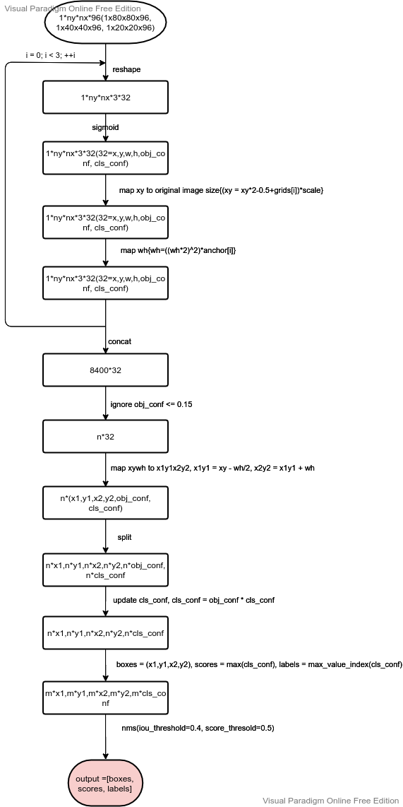
4. Post treatment

The post-processing code of YOLO v5 seems a little laborious. I sorted out the post-processing flow chart for reference.

5. Performance

YOLO v5 may not have advantages over v4 in accuracy, but it has many advantages in speed (training and reasoning, especially in the training stage). In addition, engineering ability is also an advantage.

reference resources

• In simple terms, complete explanation of Yolov5 core basic knowledge of Yolo series